Miniaturizing OCT Probes: Engineering Breakthroughs for Surgery in Confined Anatomical Spaces

Abstract

This article comprehensively explores the engineering challenges and innovative solutions for Optical Coherence Tomography (OCT) probe miniaturization, essential for real-time, high-resolution imaging in minimally invasive and microsurgery. We detail the core principles and clinical drivers, evaluate diverse design methodologies including fiber-optic, MEMS, and GRIN lens-based systems, and analyze their specific applications in neurosurgery, otolaryngology, and ophthalmology. Critical troubleshooting for optical performance, mechanical robustness, and sterilization is addressed. Finally, we present a framework for validating miniaturized probe performance against clinical benchmarks and conventional systems, providing researchers and medical device developers with a roadmap for translating these advanced imaging tools from the lab to the operating room.

The Why and What: Clinical Imperatives and Core Principles of Miniaturized OCT Imaging

Technical Support Center: OCT Probe Miniaturization for Constrained Access Research

Troubleshooting Guide: Common Experimental Issues

Q1: During in situ imaging in a narrow ENT canal, our OCT probe exhibits significant signal dropout and artifact. What could be the cause? A: This is typically due to probe-tissue contact loss or excessive pressure causing deformation. Ensure the probe sheath is properly lubricated and calibrated for non-contact imaging at the correct working distance (typically 2-5 mm). Use the integrated distance sensor (if available) or a spacer. Artifacts like "shadows" often indicate blood or other fluid ingress; consider using a saline flush channel or a disposable, clear sheath.

Q2: Our miniaturized forward-looking OCT probe shows degraded axial resolution in deep neurosurgical phantom models despite specifications. How do we troubleshoot? A: First, verify the probe's performance in a controlled test medium (e.g., water). Degradation in phantoms is often due to scattering mismatches. Confirm the phantom's scattering coefficient (µs) matches the target tissue (~5-15 mm⁻¹ at 1300 nm). Re-calibrate the reference arm. If using a MEMS scanner, ensure driving voltages are stable, as fluctuations can distort scans.

Q3: In pediatric procedure simulations, our probe’s bending radius causes fiber breakage or signal loss. What is the solution? A: You are likely exceeding the minimum bend radius of the optical fiber. For single-mode fibers at 1300 nm, the safe bend radius is often >15 mm. Solutions: 1) Use specialized bend-insensitive fiber (e.g., Corning ClearCurve). 2) Re-design the probe's articulation section with a dedicated support spine. 3) Implement a sacrificial, replaceable flex sheath that bears the mechanical stress.

Q4: How do we maintain sterility while using a research-grade OCT probe in a simulated surgical field? A: Use a FDA-cleared, sterile, single-use disposable sheath that is optically clear at your operating wavelength. Ensure the sheath does not introduce additional optical interfaces that create ghost reflections. For the probe body itself, a sterile plastic drape with a custom adapter port is recommended. Always validate imaging performance with the sheath prior to experimentation.

Frequently Asked Questions (FAQs)

Q: What are the key quantitative benchmarks for OCT probe dimensions in constrained surgical access? A: See Table 1 for current benchmarks based on anatomical access routes.

Table 1: Anatomical Access Constraints & OCT Probe Targets

Surgical Field	Typical Access Pathway Diameter (mm)	Critical Bend Radius (mm)	Target OCT Probe Outer Diameter (OD)	Required Field of View (mm)
Neurosurgery (Deep Brain)	3-5 (via port)	≥25	<2.5 mm	3-5
ENT (Sinonasal)	2-4	≥15	<1.8 mm	4-6
Pediatric (Airway, Neonatal)	1.5-3	≥20 (gentle)	<1.2 mm	2-4

Q: What is the standard protocol for characterizing a new miniaturized OCT probe's performance? A: Protocol: Bench-Top Characterization of Miniaturized OCT Probes.

• Resolution Measurement: Image a USAF 1951 resolution target. Use a 5% knife-edge method in air and in scattering medium (e.g., 1% intralipid) to measure lateral and axial resolution.
• Sensitivity Roll-off: Place a mirror at the focal point. Record peak signal (in dB) as the mirror is moved through the depth range. Plot signal vs. depth. A drop of >6 dB over 2 mm is unacceptable for most tissue imaging.
• Bend Loss Test: Secure the probe in a calibrated jig. Measure output power (dBm) while incrementally decreasing the bend radius from 50 mm to 5 mm. Record the radius where loss exceeds 0.5 dB.
• Sterilization Cycling: Subject the probe/sheath assembly to 3 cycles of low-temperature hydrogen peroxide plasma (e.g., STERRAD). Re-test resolution and sensitivity.

Q: Which signaling pathways are most relevant for functional OCT in constrained oncology access? A: In narrow-access surgical oncology (e.g., pituitary tumors, laryngeal cancer), angiogenic and hypoxic pathways are key. OCT angiography (OCTA) visualizes microvasculature, while spectroscopic OCT can infer hypoxia.

(OCT-Angiography & Hypoxia Signaling Pathway)

Q: What is the typical workflow for validating a probe in a surgical phantom? A:

(Probe Validation in Surgical Phantom Workflow)

The Scientist's Toolkit: Research Reagent Solutions

Table 2: Essential Materials for Constrained-Access OCT Research

Item	Function	Example/Specification
Bend-Insensitive SMF	Transmits light with minimal loss in tight bends.	Corning ClearCurve; 2.5-3.0 µm mode field diameter at 1300nm.
Graded-Index (GRIN) Lenses	Enables focusing in ultra-small probes (<1mm OD).	0.25-0.5 mm diameter, pitch tailored for working distance.
MEMS Scanning Mirror	Provides distal scanning in a tiny form factor.	1D or 2D, ±10° optical angle, <1.5x1.5 mm package size.
Optical Phantom Material	Mimics tissue scattering for bench validation.	Silicone or polyurethane with TiO₂/Al₂O₃ scatterers (µs = 5-20 mm⁻¹).
Sterile Disposable Sheath	Maintains asepsis; must be optically clear.	Cyclic olefin copolymer (COC) tubing, AR-coated if possible.
Precision Pullback Stage	Simulates linear scanning for forward-looking probes.	Motorized, <10 µm resolution, for in vitro vessel/phantom scans.
Low-Temperature Sterilant	For probe re-use between experiments on biologics.	Hydrogen peroxide plasma (e.g., STERRAD) or ethylene oxide gas.

Technical Support Center: Troubleshooting & FAQs for OCT Probe Miniaturization Research

This support center addresses common experimental challenges faced by researchers working on OCT probe miniaturization for constrained surgical access, as part of a broader thesis in this field.

Frequently Asked Questions (FAQs)

Q1: During in-vivo testing of our miniaturized TD-OCT probe, we observe significant signal attenuation and poor penetration depth. What are the primary causes? A: In Time-Domain (TD) OCT systems, signal attenuation in miniaturized probes is often due to limited optical power delivery from the reference arm and misalignment in the miniature interferometer. Ensure your broadband source power is sufficient (>5 mW typical) and that the optical path in the probe is free of bends below the fiber's minimum bend radius. Check for coupling losses at each micro-optical component interface.

Q2: Our lab-built SD-OCT system for endoscopic use shows pronounced side lobes (artifacts) in the axial point spread function (PSF), reducing image clarity. How can this be corrected? A: Side lobes in Spectral-Domain (SD) OCT are typically caused by non-Gaussian shape of the light source spectrum or irregularities in the spectrometer's detector array. To correct:

• Characterize your source spectrum with an optical spectrum analyzer. Apply a numerical spectral shaping (apodization) window (e.g., Hamming, Hann) to the acquired k-space data before FFT.
• Calibrate the spectrometer's wavelength-to-pixel mapping using a known gas cell (e.g., HCN) for absolute calibration, or a tunable laser for relative calibration, to ensure linear sampling in k-space.

Q3: The imaging range of our miniaturized SS-OCT system is unexpectedly limited, causing aliasing. What system parameters should we re-evaluate? A: The maximum imaging range (zmax) in Swept-Source (SS) OCT is defined by zmax = λc² / (4n Δλ), where λc is the central wavelength, n is the refractive index, and Δλ is the sweep bandwidth. Aliasing occurs when the sample structure exceeds this range. To fix:

• Increase the sweep bandwidth (Δλ) of your laser if possible.
• Digitize the interferometric signal at the correct sampling rate, ensuring it is triggered by the laser's intrinsic k-clock to maintain linearity in wavenumber.
• Confirm that the data acquisition card's sampling depth (bits) is sufficient for the dynamic range of your signal.

Q4: When integrating a miniaturized GRIN lens-based probe, we notice severe astigmatism and asymmetric resolution. What is the likely assembly issue? A: This indicates a tilt and/or de-centering between the single-mode fiber core and the GRIN lens axis. Use an active alignment station:

• Collimate light from the fiber and project it onto a 4-quadrant detector or a CCD camera.
• While monitoring the spot's centroid and circularity, adjust the 5-axis (X, Y, Z, Pitch, Yaw) position of the fiber until the collimated beam is symmetric and centered.
• Use UV-curing adhesive with a low shrinkage formula (<2%) to fix the alignment, curing in stages to minimize drift.

Troubleshooting Guides

Issue: Depth-Dependent Signal Roll-Off in SD-OCT System Symptoms: Signal strength decreases rapidly with imaging depth, limiting usable range. Diagnosis & Steps:

• Check Spectrometer Resolution: The spectrometer's limited line width (pixel resolution) causes a decay in the Fourier transform. Measure the system's sensitivity roll-off by imaging a mirror at varying path length differences.
• Verify Source Coherence Length: Ensure your superluminescent diode (SLD) has a coherence length longer than your desired imaging range.
• Re-calibrate k-Space Linearization: Non-linear sampling in k-space accelerates roll-off. Re-acquire calibration data and apply the correct interpolation algorithm to resample data into linear k-space.

Issue: Relative Intensity Noise (RIN) in SS-OCT Images Symptoms: High-frequency vertical striping or granular noise in cross-sectional images, independent of sample. Diagnosis & Steps:

• Implement Balanced Detection: Replace single detector with a balanced receiver. This subtracts common-mode noise from the source.
• Optimize Laser Operating Point: RIN is highest at the edges of the sweep. Software-trim the acquired sweep to use the central 80% where RIN is lower.
• Apply Numerical RIN Subtraction: Acquire a background spectrum (block sample arm) and subtract it from each A-scan during processing.

Quantitative System Comparison

Table 1: Key Performance Parameters of OCT System Architectures

Parameter	Time-Domain (TD) OCT	Spectral-Domain (SD) OCT	Swept-Source (SS) OCT
Typical Axial Resolution	5-15 µm in tissue	3-8 µm in tissue	4-10 µm in tissue
Imaging Speed (A-scan rate)	Slow (Hz - kHz)	Very Fast (10 - 500 kHz)	Fast to Very Fast (20 kHz - 10+ MHz)
Maximum Imaging Range	Limited by reference arm scan	~1-3 mm (limited by spectrometer)	5 - 20+ mm (limited by laser coherence)
Key Noise Source	Shot noise, thermal noise	Shot noise, sensitivity roll-off	Relative intensity noise (RIN)
Probe Miniaturization Suitability	Moderate (requires moving mirror)	High (all-fiber, static interferometer)	High (all-fiber, simplified detection)
Common Light Source	Broadband SLD	Broadband SLD or Supercontinuum	Tunable Laser (Swept Source)

Table 2: Common Artifacts & Corrections in Miniaturized Probes

Artifact	Likely Cause	Correction Protocol
Fan-shaped Distortion	Non-telecentric scan from MEMS mirror	Use a corrective scanning lens or apply image warp calibration using a grid target.
Signal Dropout	Fiber bending loss below critical radius	Re-route fiber optic cabling to maintain bend radius > 15mm for SMF-28e.
Ghost Images	Back-reflection from probe lens surfaces	Index-match lens interfaces or apply anti-reflective (AR) coatings optimized for the central wavelength.
Uneven Illumination	Misaligned fiber to collimator in sample arm	Re-align using shearing interferometry or knife-edge technique to achieve Gaussian beam profile.

Experimental Protocols

Protocol 1: Calibration of Spectrometer in a Bench-Top SD-OCT System Purpose: To achieve linear sampling in wavenumber (k-space) for optimal resolution and signal roll-off performance. Materials: SD-OCT system, Mercury-Argon (HgAr) calibration lamp, optical fiber coupler. Methodology:

• Direct the fiber output from the sample arm towards the HgAr lamp's emission, coupling the light back into the system.
• Acquire raw spectrometer data (intensity vs. pixel index) with the reference arm blocked.
• Identify the known spectral peaks of HgAr (e.g., 435.8 nm, 546.1 nm, etc.) in the pixel data.
• Fit a polynomial (typically 3rd-5th order) to map pixel index to precise wavelength (λ).
• Convert wavelength to wavenumber (k = 2π/λ) and interpolate the raw data to be evenly spaced in k.
• Save this calibration map for real-time processing of all subsequent A-scans.

Protocol 2: Characterizing Lateral Resolution of a Miniaturized OCT Probe Purpose: To empirically measure the lateral point spread function (PSF) and resolution of a custom miniaturized probe. Materials: Miniaturized probe on alignment stage, USAF 1951 resolution test target, translation stages (X, Y, Z), data acquisition computer. Methodology:

• Mount the probe perpendicular to and facing the USAF target.
• Align the probe's beam to be normal to the target surface using the reflection from the target.
• Acquire a 3D volume scan of the target, ensuring groups of bars are within the field of view.
• Reconstruct en-face (XY) images at the focus depth.
• Identify the smallest set of bars where the pattern is resolvable (contrast > 26.4% per Rayleigh criterion).
• Calculate line width per the USAF group/element specification. Alternatively, scan a sharp edge (e.g., razor blade) and measure the 10-90% intensity transition distance to determine beam spot size.

Visualizations

SD-OCT Spectrometer Calibration Workflow

Key Components of a Miniaturized OCT Probe

The Scientist's Toolkit: Research Reagent & Material Solutions

Table 3: Essential Materials for OCT Probe Prototyping & Testing

Item	Function/Description	Application in Probe Miniaturization
Single-Mode Optical Fiber (SMF-28e)	Provides a single spatial mode for interferometry; low dispersion at 1300nm.	Core light delivery channel for the probe. Diameter dictates minimum probe size.
Graded-Index (GRIN) Lenses	Cylindrical lenses for collimation/focusing; enable lens-to-fiber bonding.	Key for creating compact, robust optical assemblies without bulk optics.
MEMS Scanning Mirror	Micro-mirror that tilts on 1 or 2 axes to steer light.	Enables miniaturized, high-speed beam scanning inside narrow-gauge probes.
Index-Matching Gel/Epoxy	Optical adhesive with refractive index near glass/fiber (~1.46).	Bonds optical components, reduces back-reflection artifacts at interfaces.
USA 1951 Resolution Target	Standard test pattern with groups of bars at defined spacings.	Empirically measures lateral resolution and distortion of the imaging probe.
Optical Spectrum Analyzer (OSA)	Instrument to measure power versus wavelength.	Characterizes light source spectrum (Δλ, shape) critical for axial resolution.
Fiber Optic Rotary Joint (FORJ)	Passes optical signals across a rotating interface.	Essential for side-viewing endoscopic probes that require continuous rotation.

Technical Support Center: OCT Probe Miniaturization for Constrained Surgical Access

Troubleshooting Guides

Guide 1: Addressing Severe SNR Drop in Sub-1mm Diameter Probes

Issue: After miniaturizing a spectral-domain OCT (SD-OCT) probe to a 0.8mm diameter for endoscopic use, the SNR has dropped from 98 dB to 72 dB, rendering images unusable for quantitative analysis.

Diagnostic Steps:

• Verify Source Power: Use a calibrated optical power meter at the probe tip. Ensure output is within 5-10 mW (for safe in vivo use). A drop here indicates coupling loss.
• Check Back-Reflection: Use an optical multimeter to measure back-reflection at the connector. A reading > -40 dB suggests a dirty or damaged connector, causing source power loss.
• Analyze Spectrometer: Acquire a background spectrum (with probe tip blocked). Look for non-uniformities or a lower total count, indicating grating or camera misalignment.
• Perform Roll-Off Test: Image a mirror at increasing depths. A rapid signal drop (>15 dB over 1 mm) indicates dispersion mismatch, often from using incorrect length of compensating fiber.

Resolution Protocol:

• If source power is low: Re-cleave and re-couple the source fiber to the probe using a fusion splitcer with active core alignment. Apply index-matching gel to all mechanical connections.
• If roll-off is poor: Precisely measure the length of the probe's sample arm fiber. Cut and polish a new piece of identical fiber (e.g., SMF-28e) for the reference arm to match within ±1 cm. Re-integrate and recalibrate.
• General SNR Boost: Implement a weighted spectral shaping algorithm during signal processing. Use a Hann window centered on the source's peak wavelength to reduce noise floor at the cost of minimal axial resolution broadening.

Guide 2: Correcting Spatial Resolution Degradation Post-Miniaturization

Issue: A 0.5mm diameter MEMS-scanning OCT probe shows lateral resolution of 25 µm (vs. designed 15 µm) and axial resolution of 10 µm (vs. designed 7 µm in tissue).

Diagnostic Steps:

• Measure Point Spread Function (PSF): Image a dilute solution of 1 µm polystyrene beads or a sharp, clean mirror edge.
• Lateral Resolution Check: Plot the intensity profile across a single bead. The full width at half maximum (FWHM) > design specification indicates optical aberrations.
• Axial Resolution Check: Measure the FWHM of the interferometric signal peak from the mirror surface. A broader peak indicates insufficient source bandwidth or chromatic dispersion.

Resolution Protocol:

• For poor lateral resolution: This is often due to under-filled or over-filled micro optics. If using a GRIN lens, verify its pitch (e.g., 0.25±0.01). Reposition the fiber core precisely at the lens's focal point using a V-groove assembly stage under microscopic guidance.
• For poor axial resolution: Verify the super luminescent diode (SLD) source bandwidth. It must be >100 nm centered at 1300 nm for <7.5 µm axial resolution. Replace source if degraded. Ensure no optical bandpass filters in the system are unintentionally narrowing the spectrum.

Frequently Asked Questions (FAQs)

Q1: What is the fundamental physical limit to miniaturization in OCT probes, and which parameter is most affected? A: The fundamental limit is governed by the core diameter and numerical aperture (NA) of the single-mode fiber (SMF). As probe diameter shrinks below ~0.5 mm, bending losses in the fiber increase exponentially, and manufacturing tolerances for micro-optics (lenses, prisms) become prohibitive. The Signal-to-Noise Ratio (SNR) is the most severely compromised parameter, as smaller lenses capture less backscattered light, and increased fiber bending attenuates the signal.

Q2: We are switching from a 2.0mm probe to a 0.8mm probe for rodent brain imaging. Our A-scan rate seems slower. Is this related to size? A: Yes, indirectly. Smaller probes, especially those using MEMS or piezo scanners, have a smaller mirror mass and can potentially be driven faster. However, the lower light throughput (SNR) forces you to increase the exposure time per A-scan or digitally average multiple scans to recover image quality. This reduces the effective line rate. Check your system's maximum permissible exposure power at the smaller core diameter and adjust camera integration time accordingly.

Q3: How do I choose between a GRIN lens and a compound lens for a 1mm probe? A: The choice involves a direct trade-off within the trilemma. See the table below for a quantitative comparison.

Q4: Can computational imaging solve the miniaturization trilemma? A: Not solve, but significantly mitigate. Techniques like compressed sensing allow for fewer A-scans per B-scan, enabling faster imaging with smaller probes at the same SNR. Deep learning-based denoising (e.g., using a U-Net architecture) can recover SNR from noisy, high-speed acquisitions. However, these methods require extensive training data and cannot recover information completely lost due to physical limits.

Table 1: Performance Trade-offs in Common Miniature OCT Probe Designs

Probe Type	Typical Outer Diameter	Lateral Resolution (in tissue)	Axial Resolution (in tissue)	Typical SNR (in vivo)	Best Use Case
Standard Rotary Pullback	2.4 - 3.2 mm	15 - 25 µm	7 - 10 µm	95 - 105 dB	Coronary artery imaging, large lumen GI
Distal MEMS Scanner	1.8 - 2.2 mm	20 - 30 µm	8 - 12 µm	90 - 98 dB	Forward-viewing ENT, neurosurgey cavities
GRIN Lens Probe	0.8 - 1.2 mm	18 - 25 µm	7 - 10 µm	78 - 88 dB	Rodent brain, narrow bile ducts
Compound Lens Probe	0.8 - 1.2 mm	12 - 18 µm	6 - 8 µm	70 - 82 dB	High-res retinal, cellular imaging
Ultrathin Static Imaging Fiber	< 0.5 mm	30 - 50 µm	15 - 20 µm	60 - 70 dB	Needle-based biopsy guidance

Table 2: Impact of Key Parameters on the Trilemma

Parameter Change	Effect on Size	Effect on Resolution	Effect on SNR	Mitigation Strategy
Increase Fiber NA	Enables shorter lens → Smaller probe	Higher NA improves lateral resolution	Increases dispersion, can lower SNR	Use ultra-broadband source, digital dispersion compensation.
Reduce Wavelength (e.g., to 800nm)	Optics can be smaller	Improves lateral resolution	Higher scattering in tissue → Lower SNR	Limit use to superficial tissue layers (e.g., retina).
Use DCF (Dispersion Comp. Fiber)	Increases rigidity, may increase diameter	Maintains axial resolution	Improves SNR by preserving roll-off	Precise length matching is critical; adds cost.
Implement FDML Laser	Source is external, no size impact	No direct impact	Greatly improves SNR for high speeds	Increases system cost and complexity significantly.

Experimental Protocols

Protocol 1: Systematic Characterization of a Miniature OCT Probe Performance Objective: To quantitatively measure the size, resolution, and SNR of a custom miniaturized OCT probe.

• Diameter & Rigidity: Measure outer diameter with digital calipers at 3 points. Clamp probe at base, measure deflection angle (θ) with a protractor under a 0.1N lateral load. Calculate bending stiffness.
• Axial Resolution: Immerse probe tip in water, place a mirror in the focal plane. Acquire an A-scan. The axial resolution (∆z) is the FWHM of the interference peak, calculated as: ∆z = (2 ln2/π) * (λ²/∆λ), where λ is central wavelength and ∆λ is FWHM bandwidth. Validate with measurement.
• Lateral Resolution & FOV: Image a USAF 1951 resolution target or sub-resolution beads. Measure the FWHM of the line spread function. Map the intensity of a point source across the scan range to define the usable FOV.
• SNR Measurement: Place a 99% reflective mirror in the focal plane. Acquire 100 A-scans. Calculate the mean peak signal power (S). Move mirror out of focus to measure noise power (N) in the same depth region. SNR = 10·log₁₀(S/N). Perform at multiple depths to measure roll-off.
• Sensitivity Roll-Off: Measure SNR vs. depth as in step 4. Report the depth where SNR drops by 6 dB and 20 dB from its peak.

Protocol 2: In Situ Calibration for MEMS-Based Scanning Probes Objective: To correct for nonlinear scanning and wobble in a distal MEMS scanner.

• Grid Pattern Acquisition: Fabricate a precise 2D grid pattern (e.g., etched silica). Image the grid using the MEMS probe, driving the scanner with a theoretical linear voltage ramp.
• Feature Detection: Use a centroid-finding algorithm (e.g., in MATLAB or Python with OpenCV) to locate the (x,y) position of each grid intersection in the acquired image.
• Map Creation: Create a lookup table that maps the actual pixel coordinates of each intersection to the theoretical voltage coordinates sent to the MEMS.
• Implementation: Integrate this distortion map into the scan controller's firmware or apply it as a post-processing warp to all subsequent images. Re-calibrate monthly or after any physical shock to the probe.

Diagrams

Diagram 1: OCT Miniaturization Decision Pathway

Diagram 2: Key SNR Loss Pathways in a Miniature OCT Probe

The Scientist's Toolkit: Research Reagent & Material Solutions

Item	Function in OCT Probe Miniaturization Research	Example Product / Specification
Single-Mode Fiber (SMF)	The optical waveguide; its core size and NA set fundamental limits.	Corning SMF-28e+: Standard 9µm core, low bend loss for >1mm probes. Nufern UHNA-7: High NA (0.4) for ultra-small lenses, but higher loss.
Dispersion Compensating Fiber (DCF)	Compensates for chromatic dispersion in long SMF spans, preserving axial resolution and SNR roll-off.	OFS DK-100: Negative dispersion, must be precisely length-matched to sample arm fiber.
GRIN Lens	Collimates/focuses light in a compact cylindrical form factor. Pitch determines working distance.	GRINTECH GT-LFRL-100-025-ACN: 0.25 Pitch, 1mm diameter, NIR coating. Pitch tolerance is critical.
MEMS Mirror Die	Provides 2D scanning in a micro-scale package at the distal tip.	Mirrorcle Technologies A7B-2.0: 1mm mirror diameter, bimagnetic actuation, integrated driver.
Index Matching Gel/Oil	Reduces Fresnel reflection losses at fiber-air-lens interfaces, crucial for SNR.	Thorlabs G608N3 (Gel) or nD = 1.4580 Oil. Must be low volatility and biocompatible for clinical translation.
Polystyrene Microspheres	Sub-resolution particles used as point targets for precise PSF and resolution measurement.	Thermo Scientific 4009A: 1µm diameter beads, diluted in deionized water or agarose phantom.
Optical Power Meter & Sensor	Quantifies light throughput at each stage (source, post-coupling, probe tip) to diagnose losses.	Newport 1919-R with 918D-UV-OD3R sensor. Calibrated for 800-1300nm range.
Fusion Splicer with Core Alignment	Essential for low-loss (<0.1 dB) fusion of fibers, especially when joining different fiber types (SMF to DCF).	FITEL S177A: High-precision core alignment for fibers from 80µm to 2mm cladding.

Troubleshooting Guides & FAQs

FAQ 1: My axial resolution has degraded significantly. What could be the cause and how can I troubleshoot it?

• Answer: Degraded axial resolution in a miniaturized OCT probe is most often related to the light source spectrum. First, check the spectral bandwidth output of your superluminescent diode (SLD) or swept-source using an optical spectrum analyzer. A drop in bandwidth directly reduces axial resolution. In constrained surgical probes, mechanical stress on the fiber or contamination on connectors can cause this. Clean all optical connectors. If the issue persists, the source itself may be aging and require replacement. For system calibration, ensure the reference arm path length is correctly matched to the sample arm, especially after probe handling.

FAQ 2: The lateral resolution in my images appears blurry. How do I diagnose and fix this issue?

• Answer: Blurry lateral resolution typically points to the focusing optics in the probe's distal end. For gradient-index (GRIN) lens or ball-lens-based miniaturized probes, check for:
  • Working Distance (WD) Misalignment: Ensure the sample is within the designed WD. Use a known target (e.g., a sharp edge) and translate it axially to find the point of best focus.
  • Lens Contamination: Biological or other debris on the probe's protective window or lens will scatter light. Inspect the distal tip and clean gently with recommended solvents.
  • Fiber Misalignment: Internal misalignment between the single-mode fiber and the focusing lens, potentially caused by shock, will degrade the beam waist. This often requires probe manufacturer service.

FAQ 3: My achieved scan range is smaller than the probe's specification. What steps should I take?

• Answer: A reduced field-of-view (scan range) is usually tied to the scanning mechanism. For MEMS-based probes, verify the drive voltage/current from the controller is reaching the specified level. Use an oscilloscope to check the waveform. For piezoelectric tube scanners, resonant frequency shifts can occur. Recalibrate the scanning driver's voltage and frequency settings according to the probe's datasheet. Also, ensure no physical obstructions are impeding the scanner's movement within the sealed probe housing.

FAQ 4: The A-scan rate seems unstable, causing artifacts in B-scans. How can I resolve this?

• Answer: Instability in the A-scan rate disrupts synchronization. First, ensure your data acquisition (DAQ) card's trigger signal from the OCT engine (k-clock for swept-source, trigger TTL for SD-OCT) is stable and free from noise. Use shielded cables. In miniaturized systems, long, flexible drive cables for distal scanners can introduce capacitance and signal degradation. Try shortening cable paths or using recommended amplifiers/drivers. Check for software buffer overflows in the acquisition software that may drop lines.

FAQ 5: How do I accurately measure and verify the Working Distance of my custom miniaturized probe?

• Answer: Use a precise axial translation stage and a high-reflectance target (e.g., mirror). Mount the probe pointing at the target. Acquire A-scans while moving the target through the focus. The working distance is the distance from the probe tip to the target position where the A-scan peak intensity is maximum and the full width at half maximum (FWHM) of the point spread function is minimized. Repeat across the lateral field to map WD uniformity.

Table 1: Typical Target Specifications for Miniaturized Surgical OCT Probes

Metric	Typical Target for Micro-Surgery	Primary Governing Factor	Common Challenge in Miniaturization
Axial Resolution	2 - 10 µm in tissue	Light Source Bandwidth (Δλ)	Maintaining broad bandwidth in small-diameter fibers (dispersion, bending loss).
Lateral Resolution	5 - 30 µm	Numerical Aperture (NA) of Probe Optics	Balancing high NA (good resolution) with long Working Distance and depth of focus.
Scan Range (Lateral)	1 - 4 mm (linear/arc)	Scanner Angle x Focal Length	Achieving large, linear scans with low-voltage, micro-sized actuators (MEMS, piezo).
A-scan Rate	50 - 500 kHz	Light Source Sweep/Spectrometer Rate & Scanner Speed	Data transmission over thin cables and heat dissipation in confined probe body.
Working Distance	2 - 10 mm	Lens Design (GRIN, ball, compound)	Precise optical assembly at sub-millimeter scale; stability over temperature.

Experimental Protocol: Characterization of a Miniaturized OCT Probe

Objective: To fully characterize the key performance metrics (Resolution, Scan Range, A-scan Rate, WD) of a custom-built, miniaturized OCT probe for intraoperative imaging.

Materials:

• OCT engine (SD-OCT or SS-OCT system).
• Miniaturized probe under test.
• Optical spectrum analyzer (OSA).
• Precision 3-axis translation stage with controller.
• High-reflectance planar mirror.
• USAF 1951 resolution test target or sharp-edged blade.
• Digital oscilloscope.
• Computer with OCT acquisition software.

Procedure:

• A-scan Rate Verification:
  • Connect the probe to the OCT engine. Use the oscilloscope to monitor the trigger signal for each A-scan. Measure the frequency of this signal to confirm the actual A-scan rate.

• Axial Resolution Measurement:

  • Connect the OSA to the unused port of the system's fiber coupler to sample the source spectrum. Record the central wavelength (λc) and FWHM bandwidth (Δλ).
  • Calculate the theoretical axial resolution in air: Δz = (2 ln2 / π) * (λc² / Δλ).
  • Place a mirror at the probe's approximate WD. Acquire an A-scan. Measure the FWHM of the interference peak. Convert to spatial resolution using the system's scaling factor.

• Working Distance & Lateral Resolution:

  • Mount the probe facing the mirror on the translation stage.
  • Axially translate the mirror in fine steps, recording A-scan peak intensity at each step. Plot intensity vs. distance. The distance at peak intensity is the WD.
  • Replace the mirror with a resolution target or blade. Position it at the confirmed WD.
  • Scan laterally across a sharp edge. Fit the derivative of the edge response function to an error function; the 1/e² width of the beam intensity profile is the spot size (lateral resolution).

• Scan Range Calibration:

  • Place two known, separated point targets or fine wires within the scan field at the WD.
  • Capture a B-scan. Measure the pixel distance between the target reflections.
  • Knowing the physical separation, calculate the scan range calibration factor (µm/pixel or degrees/voltage).

The Scientist's Toolkit: Research Reagent Solutions

Table 2: Essential Materials for OCT Probe Miniaturization & Characterization

Item	Function & Relevance
Single-Mode Optical Fiber (e.g., SMF-28e)	Core light delivery component; its mode field diameter dictates minimum beam waist and coupling efficiency.
GRIN Lenses & Ball Lenses	Key for miniaturized focusing optics. GRIN lenses allow cylindrical probe design; ball lenses offer simple, short focal lengths.
UV-Curing Optical Adhesive	For stable, permanent bonding of micro-optics within ferrule assemblies in constrained spaces.
MEMS Mirror Scanner	Enables fast, precise lateral beam scanning in a micro-scale package for forward-viewing probes.
Piezoelectric Tube Actuator	Provides circumferential scanning for side-viewing endoscopic probes via resonant or static actuation.
Fiber Optic Rotary Joint	Enables continuous 360-degree probe rotation for circumferential scanning in catheter-based systems.
Index-Matching Fluid/Gel	Reduces Fresnel reflections at fiber-air-lens interfaces, critical for preserving image contrast.
Precision Ferrule (Ceramic/Stylet)	Houses and precisely aligns the fiber and micro-optics at the probe's distal tip.

System Characterization Workflow Diagram

OCT Probe Characterization Steps

OCT Probe Subsystem Relationships

OCT Probe Subsystem Relationships

Thesis Context: This technical support center is framed within a research thesis on advancing Optical Coherence Tomography (OCT) probe miniaturization for constrained surgical access (e.g., neurosurgery, otology, minimally invasive procedures). The transition from benchtop to first-generation handheld probes introduces unique technical challenges addressed here.

Troubleshooting Guides & FAQs

Q1: Our first-generation handheld OCT probe shows significantly lower signal-to-noise ratio (SNR) compared to our benchtop reference system. What are the primary culprits and steps to diagnose? A1: This is a common issue due to miniaturization. Follow this diagnostic protocol:

• Check Source Coupling: Use an optical power meter at the probe's output (temporarily disconnect the sample arm). Power should be >85% of the source output. A drop indicates misalignment in the fiber-optic coupler or connector contamination.
• Benchmark with a Mirror: Replace the sample with a mirror. Acquire an A-scan. Calculate the SNR as: SNR (dB) = 20 * log10(Peak Signal / Noise Floor RMS). Compare to benchtop performance (see Table 1).
• Inspect Rotary Joint (if applicable): For side-scanning probes, rotate the joint manually while acquiring the mirror signal. Fluctuations >3 dB indicate wear or misalignment in the rotary junction, requiring replacement.
• Protocol - System SNR Measurement:
  • Materials: Mirror, index-matching fluid, optical power meter.
  • Steps: a) Align mirror at focus. b) Acquire 100 A-scans. c) Calculate mean peak intensity. d) Measure noise RMS from a region beyond coherence gate. e) Compute SNR via formula above.

Q2: We observe severe non-uniform rotational distortion (NORD) in our side-scanning handheld probe when imaging in vitro tissue phantoms. How can we quantify and mitigate this? A2: NORD arises from uneven torque transmission in the drive cable.

• Diagnosis: Image a spoke target or a phantom with known radial symmetry. Measure the angular deviation of features from their true positions.
• Mitigation Steps:
  • Ensure the drive cable is not bent below its minimum bend radius (typically 20-30mm).
  • Lubricate the sheath with a compatible fluid (e.g., saline or specific light oil).
  • Reduce rotational speed from 500 RPM to 200-300 RPM for testing.
  • Implement software-based NORD correction using a calibration scan of the spoke target to create a correction lookup table.

Q3: The field of view (FOV) in our distal-scanning MEMS-based probe is smaller than specified. What experimental tests can we run? A3: This likely relates to MEMS drive voltage or lens alignment.

• Voltage Calibration: Use a function generator to apply a slow ramp voltage to the MEMS actuator. Observe the scanning beam profile on an IR card or beam profiler. Ensure the voltage range matches the manufacturer's spec for maximum mechanical angle.
• Lens Debonding Check: Gently tap the probe head while imaging a fixed target. If the image shifts permanently, the micro-lens may be debonded, requiring repair.
• Protocol - FOV Verification:
  • Materials: USAF resolution target, kinematic mount.
  • Steps: a) Image the target. b) Identify the smallest and largest resolvable elements at the image center and edges. c) Measure the physical distance between the farthest resolvable points at the sample plane. This is your effective FOV.

Q4: How do we sterilize or disinfect a first-generation handheld probe for in vivo murine model studies without damaging it? A4: Most early prototypes are not autoclavable. Use a cold sterilization protocol:

• Wipe the distal probe tip and cable with 70% isopropyl alcohol (IPA) soaked lint-free wipes.
• For full probe disinfection, use a hydrogen peroxide plasma (e.g., STERRAD) system if compatible with probe materials (verify with manufacturer).
• Critical: Never immerse the proximal connector or rotary joint in liquid. Use a protective, sterile, transparent sheath (e.g., CIV-Flex US sheath) designed for intraoperative probes.

Table 1: Typical Performance Comparison: Benchtop vs. First-Gen Handheld Probe

Parameter	Benchtop OCT System	First-Generation Handheld Probe	Notes
Central Wavelength	1300 nm ± 10 nm	1300 nm ± 15 nm	Handheld source may have broader spectrum.
Axial Resolution	5.2 µm in air	6.5 µm in air	Degradation due to broader source bandwidth.
Lateral Resolution	8.0 µm	12-18 µm	Limited by smaller objective lens NA.
Average Output Power	4.5 mW	1.8-2.5 mW	Losses from miniaturized optics/fiber.
Typical SNR (Mirror)	105-110 dB	90-98 dB	Primary troubleshooting target.
Scan Rate (A-line)	50-100 kHz	20-50 kHz	Limited by handheld data link/speed.
Working Distance	Adjustable (10-25mm)	Fixed (2-5mm)	Designed for near-contact tissue access.
Probe Outer Diameter	N/A (Bulk System)	2.5 - 4.0 mm	Key metric for constrained access.

Table 2: Research Reagent & Essential Materials Toolkit

Item	Function/Application
USAF 1951 Resolution Target	Calibrating lateral resolution and FOV of the probe.
Index-Matching Gel	Reducing surface reflection artifacts during phantom/ ex vivo imaging.
Optical Power Meter & Sensor	Quantifying source output and detecting coupling losses in the fiber train.
Tissue-Mimicking Phantom (e.g., silicone with titanium dioxide scatterers)	Validating image quality, penetration depth, and system performance pre- in vivo use.
Sterile Probe Sheath (CIV-Flex type)	Maintaining aseptic conditions for in vivo studies with non-sterilizable probes.
Precision Kinematic Mount	Securely and reproducibly aligning phantoms or samples for comparative studies.
Fiber-Optic Cleaver & Stripper	Essential for repairing or re-terminating damaged optical fiber connections.

Experimental Protocol: Benchmarking Handheld Probe Against Benchtop Standard

Objective: Quantitatively compare key imaging metrics of a first-generation handheld OCT probe to the lab's benchtop reference system.

Materials:

• Benchtop OCT system
• First-generation handheld OCT probe
• Mirror
• USAF resolution target
• Tissue-mimicking phantom (1% intralipid or commercial equivalent)
• Optical power meter
• Index-matching fluid
• Data acquisition software

Methodology:

• System Alignment: Power on both systems 30 minutes prior for thermal stability.
• Source Power Measurement: Record source output power for both systems using the power meter.
• SNR Measurement (Mirror Test):
  • Align a mirror at the focal plane of each system using index-matching fluid.
  • Acquire 100 sequential A-scans.
  • Compute the peak signal (mean of highest 10 pixels) and noise floor RMS (from a depth region beyond coherence gate).
  • Calculate SNR in dB for both systems (see Q1 formula).
• Resolution & FOV Measurement:
  • Image the USAF target. Identify the smallest resolvable group element (where lines are distinguishable) at the center.
  • Measure the full lateral extent of the image where the target structure is visible to determine FOV.
• Phantom Imaging:
  • Image the tissue-mimicking phantom at a fixed location.
  • Measure the depth at which the signal falls to 1/e^2 of the surface signal to estimate imaging penetration depth.
• Data Compilation: Record all quantitative results in a table format (see Table 1) for direct comparison and identification of performance gaps related to miniaturization.

System Configuration & Signal Flow Diagram

Diagram 1 Title: OCT Handheld Probe System Signal Flow

Handheld Probe Internal Scanning Mechanism Diagram

Diagram 2 Title: Internal Optics of a Distal-Scanning OCT Probe

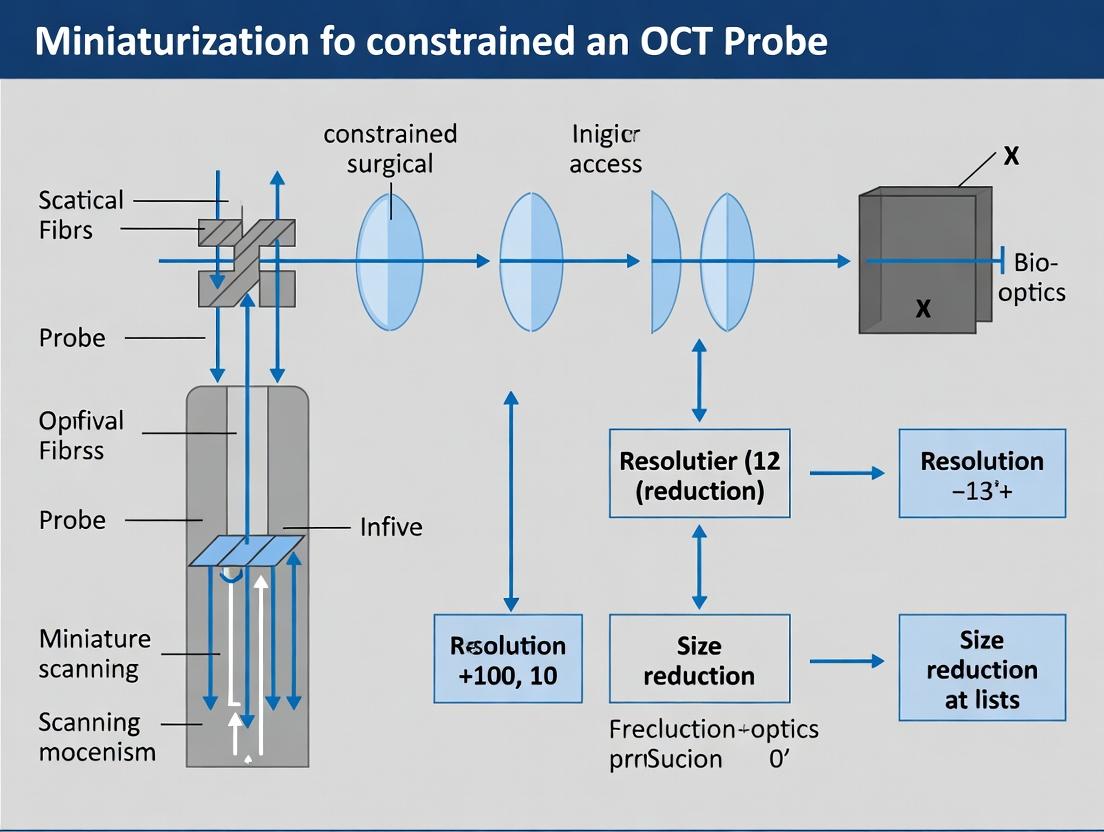
Engineering in Miniature: Design Strategies and Surgical Applications of Sub-Millimeter OCT Probes

Troubleshooting & FAQ Center

This support content is developed in the context of OCT probe miniaturization for constrained surgical access research.

Frequently Asked Questions

Q1: Our GRIN lens-based OCT probe exhibits severe astigmatism and distorted PSF. What could be the cause? A1: This is commonly caused by lens tilt or de-centering within the ferrule. GRIN lenses are sensitive to angular misalignment (>2° can cause significant aberration). Verify the assembly jig and epoxy curing protocol. Use an interferometric setup to check the wavefront pre-encapsulation. Ensure the lens is butted squarely against the fiber endface with index-matching gel before permanent fixation.

Q2: When coupling a broadband source into a hollow-core photonic crystal fiber (HC-PCF) for our micro-probe, we observe high insertion loss (>3 dB) and mode instability. How can we mitigate this? A2: This is likely due to a mismatch between the free-space Gaussian beam from your lens and the unique modal shape of the HC-PCF. Implement a free-space coupling stage with two adjustable lenses (e.g., an aspheric collimator and a microscope objective) to mode-match. Precisely align the beam to the core center using a high-precision XYZ stage while monitoring output mode profile with an IR camera. Losses below 1 dB are achievable with careful alignment.

Q3: The image quality from our fused micro-optics assembly degrades significantly after autoclaving. What material or process failure is occurring? A3: This indicates thermal expansion mismatch or epoxy degradation. Standard UV-curable epoxies have high coefficient of thermal expansion (CTE) and low glass transition temperatures (Tg). Switch to a high-temperature, low-CTE, biocompatible epoxy (e.g., EP42HT-2MED). Implement a graded thermal cycling protocol post-cure and pre-sterilization. Consider laser welding or solder glass sealing for hermetic, high-reliability assemblies.

Q4: In a dual-cladding fiber design for combined OCT/fluorescence, we get poor OCT signal when the fluorescent agent is present. Is there crosstalk? A4: Yes, this is likely fluorescence light coupling back into the single-mode OCT core, overwhelming the interferometric signal. Implement a dichroic filter at a 45° angle within the micro-assembly to physically separate the pathways. Ensure the filter's cut-on/cut-off wavelengths are precisely specified for your OCT source center wavelength and fluorescence emission band.

Troubleshooting Guides

Issue: Unstable Interferometric Signal in a Miniaturized HC-PCF Probe

• Symptoms: Fringe contrast (SNR) fluctuates rapidly, making imaging impossible.
• Probable Cause: Acoustic or thermal perturbations causing path length drift in the air-core fiber.
• Step-by-Step Resolution:
  • Isolate Vibration: Mount the probe and reference arm fiber on a vibration-isolation optical table.
  • Thermal Stabilization: Enclose the HC-PCF section in a foam sleeve to minimize air currents. Allow the system 30 minutes for thermal equilibration after power-on.
  • Source Check: Ensure your swept-source laser has a coherence length exceeding twice the probe length. Verify its relative intensity noise (RIN) specification.
  • Software Correction: Implement a real-time fringe stabilization algorithm (e.g., using a calibration mirror peak) if environmental control is insufficient in a surgical setting.

Issue: Short Working Distance in a GRIN Lens Relay Probe

• Symptoms: The designed 5mm working distance is only 2mm in practice, risking contact with tissue.
• Probable Cause: Incorrect GRIN lens parameter (pitch error) or distal protective window thickness.
• Step-by-Step Resolution:
  • Characterize Lens: Use a metric beam profiler to measure the actual beam waist location and diameter for the suspect lens batch.
  • Verify Pitch: The focusing working distance is highly sensitive to pitch (length/gradient period). A 0.05 pitch error can cause a >50% shift. Check with supplier.
  • Model Window: Re-calculate the optical path through the distal sapphire window using its exact thickness and refractive index (n~1.76 at 1300nm). Incorporate this into your ABCD matrix model.
  • Corrective Action: Adjust the spacer length between the GRIN lens and the distal window to compensate.

Experimental Protocols

Protocol 1: Characterization of a GRIN Lens for OCT Probe Design Objective: To measure the effective focal length, working distance, beam waist, and chromatic aberration of a GRIN lens at OCT wavelengths. Materials: Tunable laser source (1250-1370 nm), GRIN lens on a mount, precision translation stage, IR beam profiler camera, optical power meter, collimator. Methodology:

• Collimate the output of the tunable laser source.
• Mount the GRIN lens on a translation stage facing the collimator.
• Place the beam profiler on a separate translation stage behind the GRIN lens.
• At a central wavelength (e.g., 1310 nm), translate the beam profiler to locate the beam waist (minimum diameter). Record this position as the working distance (from lens distal face).
• Measure the beam diameter at the waist.
• Repeat steps 4-5 for wavelengths at 1250 nm and 1370 nm to assess chromatic focal shift.
• Calculate focusing performance metrics (NA, spot size).

Protocol 2: Splicing Single-Mode Fiber to Hollow-Core PCF with Low Loss Objective: To achieve a stable, low-loss (<1.5 dB) fusion splice between a standard SMF and an HC-PCF for probe assembly. Materials: Standard fusion splicer (e.g., FITEL S183A with specialized programs), SMF-28e fiber, HC-1060 (or similar) fiber, cleaver, stripping tools. Methodology:

• Cleave SMF: Standard cleave for a flat endface.
• Cleave HC-PCF: Use the "scribble-and-break" technique under a microscope to achieve a clean, core-intact endface. Avoid touching the exposed air-core microstructure.
• Splicer Setup: Use the splicer's "Hollow Fiber" or "Specialty Fiber" program. These typically use low arc power and short duration to avoid collapsing the air holes.
• Alignment: Manually adjust the core alignment using the splicer's view screen. Perfect core concentricity is critical.
• Fusion: Execute the splice. Visually inspect for no hole collapse at the splice point.
• Test: Measure insertion loss via cut-back method and inspect output mode profile for purity.

Data Presentation

Table 1: Performance Comparison of Miniaturized OCT Front-End Optics

Parameter	GRIN Lens Relay (0.25 Pitch)	Fused Silica Micro-Lens	Hollow-Core PCF + Distal Lens	Target for Neurosurgical Access
Outer Diameter (µm)	350	500	320 (fiber cladding)	< 500
Working Distance (mm)	0.5 - 5 (adjustable)	2.0	1 - 10 (via distal lens)	2 - 5
Spot Size (µm @ 1.3 µm)	15 - 25	12 - 18	10 - 20	< 25
Estimated Loss (dB)	1.5 - 2.5	1.0 - 2.0	3.0 - 6.0 (coupling + propagation)	< 3.0
Rigidity/Flexibility	Rigid relay	Rigid	Highly Flexible	Semi-flexible
Key Advantage	Simple, monolithic design	Excellent aberration control	No distal optics, immune to SNR fade	Application-dependent
Primary Challenge	Chromatic aberration, fixed WD	Precision mounting required	High coupling loss, mode instability	Reliability in sterilization

Diagrams

Diagram Title: GRIN Lens OCT Probe Assembly Workflow

Diagram Title: HC-PCF Coupling & Mode Analysis Logic

The Scientist's Toolkit: Research Reagent Solutions

Table 2: Essential Materials for Front-End Optic Assembly & Testing

Item	Function & Rationale	Example/ Specification
High-Temp Biocompatible Epoxy	For hermetic, sterilizable bonding of optics. Low CTE minimizes thermal stress.	Masterbond EP42HT-2MED (n=1.56, Tg>95°C)
Index-Matching Gel/UV Glue	Temporarily fixes components for active alignment and reduces Fresnel reflections at interfaces.	Thorlabs G608N3 (n=1.608 @ 1300nm)
Precision Alignment Station	Multi-axis (XYZ + tilt) stages with sub-micron resolution for active/passive alignment of micro-optics.	Newport 561D-XYZ with fiber rotators
IR-Sensitive Beam Profiler	Visualizes near-IR beam waist, mode profile, and divergence critical for characterizing micro-optics performance.	Ophir Pyrocam III or Xenics Bobcat-640-GigE
Broadband OCT Source	Provides the swept or low-coherence light for system testing. Bandwidth determines axial resolution.	Axsun Swept Source (100nm BW @ 1310nm)
Optical Spectrum Analyzer (OSA)	Measures source spectrum, fiber transmission spectra, and identifies loss bands (e.g., from water absorption in HC-PCF).	Yokogawa AQ6370D
Fusion Splicer (Specialty Programs)	For splicing dissimilar fibers (SMF to HC-PCF) with minimized collapse of microstructures.	FITEL S183A with "Hollow Fiber" menu

Technical Support Center

Troubleshooting Guides & FAQs

Q1: During in vivo imaging with a distally-actuated MEMS scanning probe, the scanned field of view (FOV) appears distorted and unstable. What could be the cause and how can I resolve it?

A: This is a common issue related to environmental interference on the micro-actuator. Proceed with this diagnostic protocol:

• Check Electrical Interference: Ensure all shielding on the probe drive cables is intact. Route cables away from power sources and electrosurgical units. Use a Faraday cage if possible during bench testing.
• Monitor Thermal Drift: Distal actuators, especially electrothermal MEMS, are sensitive to ambient temperature changes. Allow the system to thermally equilibrate for 30 minutes pre-experiment. Implement a closed-loop temperature control system for the probe housing if available.
• Protocol for Stability Testing:
  • Mount the probe rigidly on a bench.
  • Image a static, reflective target (e.g., a mirror or USAF target).
  • Capture sequential B-scans over 10 minutes.
  • Analyze the standard deviation of the peak position in the axial profile. A shift > 2 pixels indicates instability.
  • Solution: If instability is confirmed, recalibrate the drive voltage-to-angle lookup table in a temperature-controlled environment.

Q2: The signal amplitude in my piezoelectrically-actuated, proximally-scanned OCT probe drops significantly when the fiber is bent to navigate a surgical path. How do I diagnose and fix this?

A: This indicates bending-induced loss (macro-bending) in the single-mode optical fiber, a critical challenge in proximal actuation for constrained access.

• Diagnostic Steps:
  • Use an optical power meter to measure throughput at the probe tip with the fiber in straight and bent configurations.
  • Identify the minimum bend radius (typically < 15mm for SMF-28e) where loss exceeds 0.5 dB.
• Experimental Protocol for Characterization:
  • Setup: Couple a stable 1300nm source into the probe fiber. Measure output power at the tip.
  • Method: Coil the fiber to form loops of decreasing radius (from 40mm to 10mm in 5mm steps). Record power at each radius.
  • Analysis: Plot normalized power vs. bend radius. This characterizes your specific fiber's tolerance.
• Solutions:
  • Use bend-insensitive fiber (e.g., Corning ClearCurve) for all future probe assemblies.
  • In existing setups, ensure all bends during surgical navigation are as gentle and large-radius as possible. Use rigid or semi-rigid sleeves for critical sections.

Q3: My electrothermally-actuated MEMS scanner shows a reduced scanning angle over time, requiring increased drive voltage for the same FOV. What is happening?

A: This suggests material fatigue or degradation in the electrothermal actuator. Electrothermal mechanisms rely on differential thermal expansion, and repeated heating/cooling cycles can lead to creep or delamination.

• Accelerated Lifetime Test Protocol:
  • Drive the scanner at its maximum rated voltage (100% duty cycle, square wave) in a lab environment.
  • Periodically (e.g., every 5 hours) measure the scanning angle using a calibrated position-sensing detector (PSD).
  • Plot scanning angle vs. cumulative actuation time. A 15% drop defines end-of-life.
• Mitigation Strategies:
  • Operational: Never exceed the manufacturer's recommended maximum voltage or temperature. Use pulsed drive modes instead of continuous DC where possible to reduce average heat load.
  • Design: For next-generation probes, consider actuator materials with higher fatigue resistance like single-crystal silicon or metal alloys, though this increases fabrication complexity.

Q4: How do I choose between proximal and distal actuation for a new OCT probe design intended for intracranial surgery in rodent models?

A: The choice is governed by size constraints, required scan pattern, and durability. Use this decision framework:

Parameter	Proximal Actuation (Piezoelectric)	Distal Actuation (MEMS/Electrothermal)
Typical Outer Diameter	< 1.0 mm (limited by fiber + torque coil)	< 0.8 mm (enabled by micro-mirror at tip)
Max Scan Angle (@ 1300nm)	± 5-10 degrees (limited by fiber twist tolerance)	± 15-30 degrees (direct mirror actuation)
Resonant Frequency	100-500 Hz (for Lissajous patterns)	100-2000 Hz (highly design-dependent)
Key Advantage	Robust, sealed optical path, no electronics at distal end.	Larger FOV for given diameter, no torque-induced image distortion.
Key Limitation	FOV reduces with insertion depth due to friction/torsion.	Sensitivity to electrical noise and temperature; more complex assembly.
Best for:	Linear or slow spiral scans in fluid-filled spaces; longer probe lengths.	High-speed, precise 2D raster scans in extremely confined spaces.

Research Reagent & Essential Materials Toolkit

Item/Category	Function & Rationale
Bend-Insensitive Single-Mode Fiber (e.g., Corning ClearCurve, Nufern 1550B-HP)	Minimizes optical loss during tight bending in proximal scanning or steerable catheters, crucial for signal integrity.
UV-Curing Adhesive (e.g., NOA 86)	For lens bonding and fiber securing in probe assembly. Low shrinkage and biocompatible grades are essential.
Piezoelectric Tubing (Lead Zirconate Titanate)	The actuator for proximal scanning probes; provides rotary motion when driven by phased voltages.
MEMS Mirror Die (Custom from foundry)	The core of distal scanning; a micro-mirror actuated by electrostatic, electrothermal, or electromagnetic means.
Precision Ferrule & Sleeve	Ensures accurate and stable fiber-to-lens alignment within the probe housing.
Biocompatible Epoxy (e.g., EP30-4)	For final, hermetic sealing of the probe distal tip to prevent fluid ingress and ensure biocompatibility.
Position Sensing Detector (PSD)	Critical for characterizing scanning angle, frequency, and stability of both proximal and distal actuators.

Experimental Protocols

Protocol 1: Characterizing Scanning Linearity of an Electrothermal MEMS Actuator

Objective: To map drive voltage to actual optical deflection angle and assess linearity for image reconstruction.

• Setup: Fix the OCT probe with the MEMS scanner facing a calibrated Position Sensing Detector (PSD). Align the undeflected beam to the PSD center.
• Procedure:
  • Apply a slow ramp voltage (e.g., 0 to V_max over 10 seconds) to one axis of the scanner.
  • Simultaneously record the PSD output voltage (proportional to beam position) and the input drive voltage.
  • Convert PSD voltage to mechanical angle using the calibrated PSD sensitivity and the known working distance.
• Analysis: Plot mechanical angle (Y) vs. drive voltage (X). Fit a linear regression. The R² value quantifies linearity. Non-linearity >5% requires a correction lookup table for imaging.

Protocol 2: Measuring Resonant Frequency & Damping of a Piezoelectric Scanning Probe

Objective: To identify the resonant frequency for efficient Lissajous scanning and assess damping characteristics.

• Setup: Mount the probe tip to have free rotational movement. Attach a small, lightweight reflective flag to the ferrule. Shine a laser vibrometer beam at the flag.
• Procedure:
  • Drive the piezoelectric tube with a low-amplitude sine wave from a function generator, sweeping frequency from 10Hz to 2000Hz.
  • Use the vibrometer to record the torsional displacement amplitude and phase at each frequency.
• Analysis: Generate a Bode plot (amplitude vs. frequency). The peak amplitude identifies the resonant frequency. The width of the peak (Q-factor) indicates damping; a high Q-factor means sharp resonance, requiring precise frequency control for stable scanning.

Diagrams

Title: OCT Probe Actuation Selection Logic

Title: Electrothermal MEMS Scanner Troubleshooting Workflow

Technical Support Center

Troubleshooting Guides

Issue: Poor Signal-to-Noise Ratio (SNR) in Miniaturized OCT Probe

• Problem: Acquired A-scans/B-scans show high noise floor, obscuring biological features.
• Diagnostic Steps:
  • Check Source Power: Use a calibrated power meter at the distal end of the probe. Compare to manufacturer's specification for your light source (e.g., 850 nm SLD).
  • Inspect Coupling: Re-align the source-to-fiber coupling stage. For single-fiber systems, ensure the reference reflector (if external) is optimally aligned.
  • Fiber Integrity: Visually inspect the probe fiber tip under a microscope for cracks, burns, or contamination. Use an optical time-domain reflectometer (OTDR) if available to check for bends or breaks along the length.
  • Configuration-Specific Check:
    • Double-Clad Fiber (DCF): Verify that the cladding mode stripper is properly installed and functional. Cladding light can cause significant noise.
    • Common-Path: Ensure the reference signal from the probe tip (e.g., reflection from glass-air interface) is within the optimal range of your detector. Adjust the focus of the focusing element (GRIN lens, ball lens) if possible.
• Solution: Based on findings, re-couple the source, cleave and re-polish the fiber tip, replace the probe, or adjust the reference power in your interferometer balance.

Issue: Unstable Interferometric Fringes (Signal Fading)

• Problem: Fringe pattern or OCT image intensity fluctuates rapidly over time.
• Diagnostic Steps:
  • Environmental Vibration: Isolate the system (especially the interferometer and sample arm) from vibrations using optical breadboards and damping feet.
  • Fiber Movement: Secure all fiber patches and the probe itself. Avoid loose coils or moving sections.
  • Laser Source Stability: Monitor the source's output power and spectrum for drift. Check driver temperature and current settings.
  • Thermal Drift: Allow the system to warm up for 30-60 minutes. Check for air currents causing refractive index changes in free-space segments of the setup.
• Solution: Implement rigid mechanical mounting, use polarization-maintaining (PM) fibers if polarization fading is suspected, and ensure stable laboratory temperature.

Issue: Reduced Axial Resolution in Common-Path Probes

• Problem: Observed axial resolution is worse than theoretical calculation based on source bandwidth.
• Diagnostic Steps:
  • Source Spectrum: Measure the output spectrum directly from the probe tip using a spectrometer. Check for narrowing due to wavelength-dependent loss in fiber components.
  • Dispersion Mismatch: In common-path designs, dispersion is inherently balanced. However, if additional optical elements are added to the sample, a mismatch can occur.
  • Non-optimal Reference: In a common-path probe, the reference reflection must be strong and originate from a single, clean interface. Check for multiple parasitic reflections (e.g., from multiple lens surfaces).
• Solution: Use fibers and components with broad bandwidth specifications. Apply numerical dispersion compensation in software if a residual mismatch is characterized. Use anti-reflection coated optical elements.

Frequently Asked Questions (FAQs)

Q1: For OCT probe miniaturization in constrained surgical access (e.g., cochlea, bile duct), which fiber type is more suitable: single-mode fiber (SMF) or double-clad fiber (DCF)?

A: The choice depends on your detection scheme. For standard, lens-based focusing in a dual-arm (Michelson) interferometer, SMF is sufficient and simpler. DCF is essential only if you require simultaneous OCT imaging (via the single-mode core) and fluorescence detection/therapy (via the large, multi-mode inner cladding). For pure OCT miniaturization, SMF in a common-path configuration often provides the most robust and simplest-to-fabricate ultra-miniature probe.

Q2: What is the primary advantage of a common-path interferometer configuration for miniature probes?

A: The primary advantage is superior environmental stability. Because the sample and reference arms share the same optical path up to the probe tip, the interferometer is largely immune to vibrations, temperature fluctuations, and bending-induced path length changes in the fiber. This makes it exceptionally robust for handheld or surgically manipulated probes. It also simplifies probe construction by eliminating the need for a separate, discrete reference reflector.

Q3: How do I calculate the expected sensitivity of my fiber-optic OCT system?

A: The shot-noise limited sensitivity (in dB) is given by: Sensitivity = 10 * log10( (η * P_sample * P_reference) / (2 * P_noise) ) where η is the detector responsivity, P_sample is the power returning from the sample, P_reference is the reference arm power, and P_noise is the noise power. In practice, always measure sensitivity empirically by placing a near-100% reflector at the sample position and measuring the peak signal-to-noise ratio.

Q4: We observe "ghost images" in our common-path OCT system. What is the likely cause?

A: Ghost images are typically caused by multiple strong reflections within the probe itself. In a common-path design, the intended reference is usually the first glass-air interface at the probe tip. A second strong reflection from another surface (e.g., the connection between the fiber and the lens, or the back surface of the lens) will create a secondary, delayed interferometer, resulting in a duplicated "ghost" image. The solution is to use index-matching adhesive at all internal interfaces and/or angle polish connections to suppress these parasitic reflections.

Data Presentation

Table 1: Comparison of Single-Fiber (Common-Path) vs. Double-Clad Fiber Probes for OCT Miniaturization

Feature	Single-Mode Fiber (Common-Path)	Double-Clad Fiber (Dual-Arm Typical)
Typical Outer Diameter	125 µm (fiber only) to < 500 µm (with lens)	165 µm (fiber only) to > 600 µm (with lens)
Minimum Bend Radius	~5-10 mm (standard SMF)	~10-15 mm (stiffer due to complex structure)
Inherent Stability	Excellent (Common-path design)	Moderate (Requires separate, stable reference arm)
Multi-Modality Potential	OCT only (without complex integration)	High (OCT via core, fluorescence/ therapy via cladding)
Fabrication Complexity	Low to Moderate	High (requires splicing, cladding mode stripping)
Typical Sensitivity	100-110 dB	105-115 dB
Best For	Ultra-miniature, robust imaging-only probes	Slightly larger probes requiring combined imaging & spectroscopy/therapy

Table 2: Key Parameters for OCT Probe Design in Constrained Access

Parameter	Target Range for Micro-Surgery	Impact on Design Choice
Probe Sheath Diameter	< 1.0 mm	Drives use of bare fiber or micro-lenses; favors 125µm SMF.
Working Distance	0.5 - 2.0 mm	Determines lens selection (GRIN, ball, no lens).
Lateral Resolution	5 - 20 µm	Requires high NA focusing; may conflict with depth of field needs.
Depth of Field	1 - 3 mm	Favors lower NA optics; common-path helps maintain stability over range.
Scanning Mechanism	Proximal (fiber pull) vs. Distal (MEMS)	Common-path simplifies distal scanning by reducing wiring.

Experimental Protocols

Protocol 1: Characterizing the Performance of a Miniature Common-Path OCT Probe

Objective: To measure the axial resolution, lateral resolution, sensitivity roll-off, and sensitivity of a fabricated common-path OCT probe.

Materials: See "The Scientist's Toolkit" below.

Methodology:

• System Setup: Connect the common-path probe to the interferometer output. Ensure the spectrometer or detector is synchronized with the wavelength sweep or source modulation.
• Axial Resolution Measurement:
  • Place a mirror in a water bath (if the probe is designed for tissue imaging) at the probe's focal point.
  • Acquire an A-scan. The mirror will produce a single sharp peak.
  • Take the Fourier transform of the acquired interferogram. The full-width at half-maximum (FWHM) of the peak in the depth (axial) profile is the measured axial resolution. Compare to the theoretical resolution: Δz = (2 ln2/π) * (λ₀²/Δλ), where λ₀ is the central wavelength and Δλ is the FWHM bandwidth.
• Lateral Resolution Measurement:
  • Translate a sharp edge (e.g., a razor blade mounted on a translation stage) laterally through the probe beam at its focal plane.
  • Measure the intensity of the reflected signal as a function of edge position.
  • Take the derivative of this edge response function to obtain the line spread function (LSF). The FWHM of the LSF is the lateral resolution.
• Sensitivity & Roll-Off Measurement:
  • Place a near-perfect reflector (e.g., a silver mirror) at the probe focus.
  • Record the peak signal power (in dB) from the A-scan.
  • Gradually move the mirror away from the zero-delay position in known steps (e.g., 0.5 mm increments).
  • At each position, record the peak signal power. The decrease in signal (in dB) as a function of depth is the sensitivity roll-off. The signal at zero delay (minus the known reflector loss) gives the system sensitivity.

Protocol 2: Integrating a Double-Clad Fiber for Combined OCT and Fluorescence Sensing

Objective: To assemble and test a dual-modal probe using DCF for concurrent structural imaging (OCT) and fluorescence collection.

Materials: See "The Scientist's Toolkit" below.

Methodology:

• Fiber Preparation:
  • Cleave the DCF using a precision cleaver. Strip a section (~3 cm) of the protective coating from the distal end.
  • In the stripped section, apply a high-index polymer or epoxy to act as a cladding mode stripper, ensuring all light in the inner cladding is absorbed and does not back-propagate.
  • Splice the prepared DCF to the system's main delivery SMF using a fusion splicer with specialized programs for DCF.
• Optical Assembly:
  • Attach a micro-optic (e.g., GRIN lens) to the distal end of the DCF using UV-curing optical adhesive. Align for optimal focus.
  • At the proximal end, the DCF core is connected to the OCT interferometer. The inner cladding is coupled to a fluorescence excitation/detection path: a dichroic mirror separates excitation laser light (directed into the cladding) and emitted fluorescence (collected from the cladding and directed to a spectrometer or PMT).
• System Testing:
  • OCT Channel: Follow Protocol 1 to characterize OCT performance using the DCF core.
  • Fluorescence Channel: Place a known fluorescent target (e.g., quantum dot film) at the probe focus. Illuminate via the cladding and measure the collected fluorescence spectrum. Calculate the collection efficiency by comparing input excitation power to output fluorescence power (accounting for known target quantum yield).

Mandatory Visualization

Title: Common-Path OCT System Signal Flow

Title: Miniature OCT Probe Design Decision Workflow

The Scientist's Toolkit

Table: Key Research Reagent Solutions for Fiber-Optic OCT Probe Development

Item	Function & Rationale
Single-Mode Fiber (SMF-28e)	The standard telecommunication fiber for 1300/1550 nm OCT. Provides a robust, low-cost waveguide for the sample arm or common-path probe.
Double-Clad Fiber (e.g., DCF-13)	Enables dual-modal systems. The single-mode core carries OCT signal; the large-area inner cladding collects fluorescence or delivers therapy light.
UV-Curing Optical Adhesive (e.g., NOA 61/81)	Used for permanently bonding micro-optics (GRIN lenses, ball lenses) to fiber tips. Index-matched to glass to reduce parasitic reflections.
Index-Matching Gel	Temporarily eliminates unwanted reflections at fiber connections (e.g., between patch cords) by filling air gaps. Crucial for troubleshooting.
Precision Fiber Cleaver	Creates a perfectly flat, perpendicular end-face on optical fiber. A clean cleave is essential for low-loss connections and probe tip fabrication.
GRIN Lens (e.g., 0.25 Pitch, 0.5mm OD)	A cylindrical lens that focuses light from the fiber tip. Key for achieving a small spot size (high lateral resolution) in a miniature package.
Cladding Mode Stripper	A material (high-index polymer) applied to DCF to remove stray light propagating in the cladding, which would otherwise create noise.
Optical Spectrum Analyzer (OSA)	Measures the wavelength spectrum emitted from the probe tip. Critical for verifying source bandwidth and diagnosing system problems.
Calibrated Optical Power Meter	Measures absolute light power levels at various points in the system (source output, probe tip) to ensure optimal performance and safety.

Technical Support Center

Troubleshooting Guide & FAQs

Q1: Our miniaturized OCT probe is failing to acquire a clear A-scan signal during in vivo use. What are the primary troubleshooting steps? A: This is often related to signal-to-noise ratio (SNR) degradation. Follow this protocol:

• Check Optical Connection: Disconnect and meticulously clean all fiber optic connectors (FC/APC) with lint-free wipes and isopropyl alcohol. Ensure connectors are fully seated and the mating sleeve is not damaged.
• Verify Reference Arm Power: Use the system's internal photodetector (if available) or an external power meter to confirm reference arm power is within the manufacturer's specified range (typically 10-100 µW). Adjust if possible.
• Inspect Probe Tip: Under a microscope, examine the distal optics (GRIN lens, prism) for blood, tissue debris, or moisture. Clean gently with a sterile saline-moistened swab designed for optical components.
• Confirm Sample Positioning: Ensure the probe tip is in stable, perpendicular contact with the tissue surface or within the intended surgical cavity fluid. Use the live B-scan preview to adjust.

Q2: We observe significant image artifacts (e.g., streaking, shadows) in B-scans when imaging deep within a sulcus. What could be the cause? A: This is typically due to light-tissue interactions in constrained geometries.

• Cause 1: Multiple Scattering & Specular Reflection. The angled walls of the sulcus cause intense, direct reflections that saturate the detector and create vertical streaks.
  • Solution: Slightly tilt the probe to avoid direct back-reflection into the aperture. If the system has polarization diversity, ensure it is enabled.
• Cause 2: Signal Attenuation from Blood. Pooling of blood (highly scattering fluid) rapidly attenuates the signal.
  • Solution: Implement concurrent suction/irrigation in the access port to clear the field. Consider using a sheath with integrated irrigation for the OCT probe.

Q3: How do we validate the correlation between OCT-hypo/hyper-intensity margins and true histopathological tumor boundaries in a rodent glioma model? A: This requires a precise co-registration protocol.

• Intraoperative Marking: After OCT imaging, use a sterile surgical ink to tattoo the imaged area's boundaries (e.g., central point and cardinal directions) on the dura or cortex.
• Ex Vivo Correlation: Following sacrifice, excise the brain block with inked markers. Serially section the tissue precisely perpendicular to the OCT B-scan plane.
• Spatial Registration: Digitally map the histological section (H&E stain) to the corresponding OCT B-scan using the ink markers and major blood vessels as fiducials. Software like ImageJ with linear registration plugins is essential.

Q4: The OCT signal penetrance drops below 1 mm in our human glioma specimens, less than literature values. What experimental variables should we optimize? A: Penetrance is highly dependent on tissue preparation and system settings.

Variable	Typical Target Range	Optimization Action for Ex Vivo Specimens
Tissue Hydration	High (Physiological)	Immerse specimen in phosphate-buffered saline (PBS) during imaging. Avoid desiccation.
System Center Wavelength	~1300 nm	Confirm your system uses this optimal wavelength for tissue scattering, not 800-900 nm.
Spectral Bandwidth (FWHM)	>100 nm	Verify system calibration; a reduced bandwidth lowers axial resolution and effective signal.
Incident Power on Sample	5-10 mW	Measure directly at the probe tip. Ensure it is at the maximum safe/approved level.

Experimental Protocol: Intraoperative OCT Margin Assessment in a Murine Model

Title: Protocol for Co-registered OCT Imaging and Histopathological Validation of Glioma Margins.

Objective: To acquire in vivo OCT data from tumor margins and establish a validated correlation with post-mortem histology.

Materials:

• Orthotopic glioma model (e.g., GL261-luc in C57BL/6 mouse).
• Miniaturized OCT probe (e.g., 2.7mm outer diameter, side-scanning).
• Stereotactic frame with integrated probe holder.
• Surgical suite: drill, sterile drapes, irrigation.
• Histology setup: formalin, cryostat, microscope slides.

Methodology:

• Craniotomy & Tumor Exposure: Perform a sterile craniotomy over the tumor implantation site. Gently retract the dura to expose the cortical surface.
• OCT Probe Sterilization & Positioning: Sterilize the probe sheath with ethylene oxide. Secure the probe in the stereotactic holder. Position it perpendicular to the tissue surface, using a micromanipulator for fine control.
• Image Acquisition: Acquire volumetric OCT scans (e.g., 1000 A-scans x 500 B-scans over 4x4mm). Acquire multiple volumes from the perceived tumor core, margin, and adjacent normal tissue. Record all coordinates.
• Fiducial Marking: At key imaging sites, apply a minute drop of sterile surgical ink using a 30-gauge needle.
• Animal Perfusion & Tissue Harvest: Euthanize the animal and perform transcardial perfusion with PBS followed by 10% formalin. Carefully extract the brain, preserving orientation.
• Sectioning & Staining: Section the brain in the same plane as the OCT B-scans. Process for H&E staining and immunohistochemistry (e.g., GFAP, Ki67).
• Image Co-registration & Analysis: Use fiducial marks and vessel patterns to align OCT and histological images. Quantify OCT intensity (e.g., normalized standard deviation) within regions defined by histology.

The Scientist's Toolkit: Research Reagent & Material Solutions

Item	Function in OCT-Guided Neurosurgery Research
GRIN Lens-based Side-Firing Probe	Enables forward-viewing OCT imaging through a miniaturized (<500µm) footprint, crucial for deep surgical access.
Sterile, Single-Use Polyimide Sheath	Provides a protective barrier for the reusable OCT probe, ensuring sterility and preventing biofilm formation.
Fiducial Marking Dye (e.g., Sterile Black Ink)	Creates permanent, histology-visible reference points on tissue for accurate OCT-histology co-registration.
Artificial CSF or PBS Irrigation	Maintains tissue hydration and optical clarity during extended intraoperative imaging sessions.
3D-Printed Stereotactic Adapter	Custom-designed holder to rigidly fix the OCT probe to a surgical microscope or robotic arm for stable imaging.
Fluorescently-labeled Tumor Cells (e.g., GFP+)	Allows cross-validation of OCT-hypothesized margins with fluorescence-guided biopsy in animal models.

Visualizations

Diagram Title: OCT System Workflow for Intraoperative Imaging

Diagram Title: Tissue Contrast & Decision Logic for Tumor Margins

Technical Support Center

Troubleshooting Guides & FAQs

Q1: The OCT image appears blurry or has significant signal attenuation when imaging deep sinus cavities. What could be the cause and how can I resolve it? A: This is often caused by probe misalignment, condensation on the probe window, or insufficient probe-tissue contact in the constrained space. First, verify the probe's optical path is clear by imaging a calibration target. For in vivo use, ensure the probe's sterile sheath is properly seated and use an anti-fog solution on the distal window. For deep sinus imaging, optimize the reference arm delay and use a higher sensitivity (e.g., >100 dB) system setting. If attenuation persists, it may indicate suboptimal probe focusing for the specific anatomy; consider using a probe with a longer depth of focus.

Q2: During laryngeal imaging, we encounter motion artifacts that degrade image quality. What methodologies can minimize this? A: Laryngeal imaging is susceptible to physiological motion (respiration, pulsation) and probe motion. Implement the following protocol: 1) Use a high-speed OCT system (A-line rate >100 kHz) to "freeze" motion. 2) Synchronize data acquisition with patient respiration using a gating signal from a monitoring device. 3) Employ a probe with a distal micromotor for circumferential scanning, which stabilizes the proximal part. 4) In post-processing, apply motion correction algorithms based on image registration (e.g., phase correlation) across consecutive frames.

Q3: When navigating the narrow Eustachian tube, the probe sheath kinks, preventing advancement. Are there specific design considerations? A: Yes. This highlights the need for probe miniaturization and optimized mechanical properties. For tubal access, use a probe with a diameter ≤1.0 mm and a reinforced, torque-stable sheath. The probe's bending stiffness should be carefully engineered—too stiff risks tissue damage, too flexible causes buckling. A recommended protocol is to use a graded-stiffness guide catheter (outer) to navigate the initial curvature, followed by advancement of the more flexible OCT probe within it. Never force advancement against resistance.

Q4: We observe inconsistent image contrast between different tissue layers in the larynx. How can we improve layer differentiation? A: Inconsistent contrast can stem from suboptimal polarization matching or speckle noise. For improved layer differentiation: 1) Utilize polarization-sensitive OCT (PS-OCT) if available, as it provides birefringence contrast crucial for identifying layered structures like vocal fold epithelium and lamina propria. 2) Implement digital contrast enhancement techniques such as depth-encoded attenuation compensation or speckle variance analysis. 3) Ensure the probe's numerical aperture (NA) is appropriate; a higher NA (~0.2) provides better axial resolution for thin layer discrimination.

Q5: How do we sterilize or disinfect these miniature OCT probes for repeated clinical research use without damaging them? A: This is critical for translational research. Most endoscopic OCT probes are not autoclavable. Follow this validated protocol:

• Immediate post-procedure: Wipe the probe insertion shaft with a enzymatic cleaner.
• Leak Testing: Perform a manufacturer-specified pressure leak test before immersion.
• High-Level Disinfection (HLD): Immerse the distal tip and shaft in an FDA-approved, non-corrosive disinfectant (e.g., ortho-phthalaldehyde solution) for the exact recommended contact time (typically 5-12 minutes).
• Rinsing: Rinse thoroughly with sterile water to remove all chemical residues.
• Drying: Air dry in a sterile, protected environment. Store the probe with the distal tip protected in a coiled position to avoid fiber breakage.

Table 1: Performance Specifications of Endoscopic OCT Probes for Constrained Anatomy

Anatomical Site	Recommended Probe Diameter (mm)	Typical Scan Range (mm)	Axial Resolution (µm)	Optimal A-line Rate (kHz)	Key Challenge
Sinus Cavities	1.5 - 2.5	Radial: 5-10, Linear: 20	5 - 15	50 - 200	Navigation past turbinates, mucus interference
Larynx	1.0 - 2.0	Radial: 8-12	7 - 20	100 - 500	Motion artifacts, access past epiglottis
Eustachian Tube	0.8 - 1.2	Linear: 10-15	<10 (high res)	20 - 100	Extreme miniaturization, sterilizability

Table 2: Common Artifacts and System-Level Solutions

Artifact Type	Probable Cause	System Check	Software/Post-Processing Fix
Circular Stripes	Coherence noise from reflectors in system optics	Check collimation of source into fiber, clean all connectors.	Apply background subtraction (average of first 100 A-lines).
Depth-Dependent Signal Roll-off	Dispersion mismatch, limited spectrometer resolution	Re-balance reference arm power, optimize spectrometer alignment.	Apply digital dispersion compensation and roll-off correction algorithms.
Non-Uniform Rotation Distortion (NURD)	Friction in rotating fiber joint, cable winding	Ensure probe is straight, check torque of distal motor.	Use angular encoder data for angular remapping, if available.

Experimental Protocol:Ex VivoValidation of Miniaturized OCT Probe for Tubal Imaging

Objective: To validate the imaging performance and navigability of a sub-1mm OCT probe within a simulated Eustachian tube environment.

Materials: See "The Scientist's Toolkit" below. Methodology:

• Tissue Phantom Preparation: Create a anatomically accurate phantom using a 3D-printed mold (based on CT data) and silicone elastomer. Embed scattering agents (TiO2) to mimic tissue scattering (µs' ~5-10 mm⁻¹).
• Probe Calibration: Image a USAF resolution target and a known reflectance mirror to measure system point spread function (PSF), sensitivity roll-off, and lateral resolution.
• Navigation Test: Under a surgical microscope, navigate the probe through the phantom's narrowest segment (isthmus, ~1mm diameter). Record the force applied using a micro-force sensor attached proximally.
• Image Acquisition: Acquire 3D OCT data sets (500 x 500 A-lines) at three key locations: proximal tube, isthmus, and distal opening.
• Analysis: Quantify signal-to-noise ratio (SNR) and contrast-to-noise ratio (CNR) between the "luminal surface" and "submucosal" phantom layers at each location. Compare navigation force to established safety thresholds.

The Scientist's Toolkit: Research Reagent Solutions

Table 3: Essential Materials for Endoscopic OCT Research in Constrained Access

Item	Function & Rationale
TiO2 or Polystyrene Microsphere Phantom	Provides a stable, standardized target for calibrating system resolution and sensitivity before/after experiments.
Optical Index Matching Gel	Applied between probe and sterile disposable sheath to minimize parasitic reflections that cause image artifacts.
FDA-Cleared High-Level Disinfectant (e.g., CIDEX OPA)	For safe reprocessing of probes in translational clinical research, ensuring patient safety and probe longevity.
Torque-Stable Sheath/Guide Catheter	Enables transmission of rotational force for precise probe navigation in tortuous anatomy without kinking.
Anti-Fog Solution (Sterile)	Prevents condensation on the distal probe window when introduced into warm, humid body cavities (e.g., sinus, larynx).
Micro-Fore Sensor (e.g., Fiber Bragg Grating based)	Quantifies insertion forces during navigation experiments, providing critical data for probe safety evaluation.

Diagrams

Diagram 1: Endoscopic OCT System Workflow for Constrained Access

Diagram 2: Probe Selection Logic for Target Anatomy

Troubleshooting & Technical Support Center

Frequently Asked Questions (FAQ)

Q1: My forward-viewing needle probe exhibits significant signal attenuation in the distal 2mm of the A-scan. What are the likely causes and solutions? A: This is typically caused by misalignment of the GRIN lens or optical fiber within the hypodermic needle casing, or by fluid ingress.

• Solution 1: Verify probe integrity using an optical power meter at the connector. A drop >50% from baseline indicates internal damage. Refer to recalibration protocol.
• Solution 2: Perform a bench-top beam profile scan (see Experimental Protocol 1). A lateral shift >10% of the beam diameter indicates misalignment requiring factory repair.
• Preventive Action: Always flush the probe sheath with 70% isopropyl alcohol and dry with pressurized air after use in biological tissue.

Q2: After integration with a robotic arm, my OCT images show periodic striping artifacts. How can I diagnose the source? A: This is commonly an electrical noise issue from the robotic motors interfering with the OCT spectrometer or laser source.

• Solution 1: Physically separate the OCT engine and computer from the robotic power supplies. Use ferrite cores on all data and power cables.
• Solution 2: Run the robotic arm through its motion protocol with the OCT laser off but detection active. If artifacts persist, the interference is on the detection line. Isolate the spectrometer with a dedicated uninterruptible power supply (UPS).
• Experimental Adjustment: Implement synchronized acquisition where the OCT trigger is gated to the robot's motion controller during stationary phases.

Q3: The adhesive securing the fiber within my custom probe fails during autoclave sterilization (121°C). What are biocompatible, high-temperature alternatives? A: Standard epoxies (e.g., EPOTEK 353ND) degrade at sustained temperatures above 100°C.

• Recommended Solution: Use a sol-gel based ceramic adhesive (e.g., Ceramabond 835). It is biocompatible, provides strong bonds to glass and metal, and withstands temperatures exceeding 400°C.
• Protocol: Follow manufacturer instructions for thin-layer application. Curing requires heating to 150°C for 1 hour, which must be completed before integrating any polymer-based components like the drive cable.

Q4: When scanning through a surgical tool's channel, I observe ghost reflections that obscure the tissue surface. How can I mitigate this? A: These are parasitic reflections from the inner wall of the metallic tool channel.

• Solution 1: Apply an index-matching gel to the exterior of the probe's protective sheath before insertion into the tool channel. This reduces the refractive index mismatch.
• Solution 2: If designing a custom tool, specify a blackened, anodized, or textured inner surface to scatter reflected light.
• Software Solution: Acquire a baseline "background" scan with the probe in the tool channel facing air. Subtract this scan from subsequent in vivo scans during post-processing.

---

Experimental Protocols

Experimental Protocol 1: Beam Profile Characterization for Forward-Viewing Needle Probes Objective: Quantify beam waist, working distance, and lateral resolution to confirm probe specifications or diagnose misalignment.

Materials: See Research Reagent Solutions table.

Methodology:

• Mount the probe on a 3-axis translation stage perpendicular to a calibrated, cleaved single-mode fiber (SMF-28) acting as a point reflector.
• Connect the probe to a swept-source OCT (SS-OCT) system (e.g., Axsun, 1310nm center wavelength).
• Align the probe tip to the reflector using stage micrometers until a maximum signal is observed on the OCT M-scan display.
• Perform a 2D lateral raster scan over a 500µm x 500µm area with a 10µm step size at the suspected beam waist location.
• At each point, record the peak amplitude of the A-scan reflection from the point reflector.
• Fit the resulting 2D amplitude map to a Gaussian function: I(x,y) = I₀ * exp(-2((x-x₀)²+(y-y₀)²)/w²), where w is the 1/e² beam radius.
• Repeat the raster scan at different axial (Z) positions to plot beam radius vs. distance and locate the beam waist.

Experimental Protocol 2: Calibration of Probe Bending for Integrated Robotic Steering Objective: Map motor encoder positions to actual probe tip deflection for closed-loop control.

Methodology:

• Secure the integrated robotic tool probe in a fixture. Under a high-resolution microscope, position a grid target (100µm spacing) in the probe's field of view.
• Command the robotic actuators to bend the probe in 0.5mm increments based on internal encoder feedback, up to the maximum specified bend (e.g., 5mm).
• At each commanded position, capture an OCT B-scan. Use cross-correlation of the grid target image to measure the actual lateral displacement of the FOV in pixels.
• Convert pixel displacement to physical displacement using the grid calibration.
• Create a lookup table mapping Commanded Actuator Displacement (mm) to Actual Tip Displacement (mm) and OCT FOV Shift (degrees).

---

Data Presentation

Table 1: Performance Comparison of Miniaturized OCT Probe Designs for Surgical Access

Probe Characteristic	Forward-Viewing Needle (GRIN-based)	Side-Viewing Rotary Pullback	Integrated Robotic Tool (Steerable)
Typical Outer Diameter	22-30 Gauge (720µm - 330µm)	18-22 Gauge (1.27mm - 720µm)	2.0mm - 5.0mm (Tool Dependent)
Scanning Mechanism	Distal MEMS Mirror	Proximal Motor Rotary Pullback	Robotically Actuated Bending
Field of View	70° - 90° Conical	360° x 10mm (Radial x Longitudinal)	0° - 90° Adjustable Sector
Typical Axial Resolution	8 - 15 µm in tissue	8 - 15 µm in tissue	8 - 15 µm in tissue
Key Advantage	True forward vision, no pullback needed	Full circumferential imaging	Direct tool-tissue visualization
Primary Challenge	Limited scan area, fragile distal optics	Non-coherent rotation distortion	Calibration drift, motion artifacts

Table 2: Research Reagent Solutions for OCT Probe Development & Testing

Item	Function	Example Product / Specification
Index-Matching Gel	Reduces parasitic reflections at optical interfaces.	Thorlabs G608N3 (n=1.458 at 1310nm)
UV-Curing Adhesive	For rapid fiber lens bonding in prototyping.	NOA 81 (Biocompatible, low shrinkage)
Ceramic Adhesive	High-temperature, metal-glass bonding for sterilization.	Aremco Ceramabond 835
Single-Mode Optical Fiber	Core component for interferometric sensing.	Corning SMF-28 Ultra (9µm mode field @1310nm)
GRIN Lens	Collimates/focuses light in confined spaces.	Grintech GmbH, SLW-2.0 (0.5mm dia.)
Calibration Phantom	Validation of resolution & signal penetration.	ATS Labs Multi-Modal Phantom (0.5% Intralipid)
Fluoroethylene Polymer (FEP)	Low-refractive-index, biocompatible sheathing.	Zeus FEP Heat Shrink Tubing (n=1.338)

---

Visualizations

Diagram 1: OCT Needle Probe Troubleshooting Workflow

Diagram 2: Robotic OCT System Integration Pathway

Overcoming Miniaturization Hurdles: Solving Optical, Mechanical, and Clinical Deployment Challenges

Troubleshooting Guides & FAQs

This technical support center addresses common mechanical failure modes in miniaturized OCT probes for constrained surgical access research. The following guides help diagnose and mitigate issues during in-vitro and preclinical experiments.

FAQ 1: My OCT probe’s SNR has degraded significantly after repeated flexing in a mock surgical channel. What is the likely cause and how can I test it?

• Answer: This is a classic symptom of reduced flex life leading to optical fiber fatigue or micro-bending losses. To test:
  • Isolate the Bend: Use a motorized flexion jig to replicate the exact bend radius (R) and cycle count (N) from your experiment.
  • Measure Baseline & Post-Flex Attenuation: Use an optical power meter at the probe’s output. A power drop >1 dB typically indicates failure.
  • Inspect: Use micro-CT or microscopy to identify fiber cracks or sheath breaches.

FAQ 2: During rotational scanning within a rigid guide cannula, my probe’s rotation becomes non-uniform, causing image artifacts.

• Answer: This suggests insufficient torque resistance or binding.
  • Check Friction: Measure the rotational torque required at the proximal end using a torque gauge. A sudden increase indicates internal binding.
  • Inspect for Kinks: A localized kink will cause a drastic torque increase. Visually inspect the probe along its length.
  • Verify Drive Consistency: Ensure your rotary pullback motor provides constant angular velocity under load. Test with a known-good, stiff dummy fiber.

FAQ 3: How can I quantify the kink resistance of different probe designs before animal studies?

• Answer: Implement a standardized kink-test protocol.
  • Tool: Use a force gauge with a radius mandrel.
  • Method: Form a loop of a controlled diameter (e.g., 5mm) and measure the force required to further reduce the loop radius by 1mm.
  • Metric: Record the force at which a >3dB drop in optical transmission occurs. This is the kink threshold.

FAQ 4: The protective sheath of my probe has buckled during advancement, preventing access to the target site.

• Answer: This is a failure in compressive column strength, often related to sheath material and wall thickness.
  • Immediate Mitigation: Ensure the probe is advanced through a stabilized guide tube. Never push an unsupported, long, thin probe.
  • Design Test: Perform a column crush test. Fix the probe horizontally, apply axial compressive force via a force gauge, and measure displacement. Compare designs quantitatively.

Table 1: Flex Life Performance of Common Probe Sheathing Materials

Material	Typical Wall Thickness (µm)	Mean Cycles to Failure (R=5mm)	Failure Mode
Polyimide Tubing	25-30	>100,000	Fiber fracture
Heat-Shrink PTFE	50	~20,000	Sheath cracking
Stainless Steel Coil	75 (OD)	>500,000	Note: Virtually infinite, but may transfer stress to inner components.
Polyether Block Amide (PEBAX)	100	50,000	Plastic deformation, hysteresis

Table 2: Torque Transmission Efficiency of Different Drive Configurations

Drive Configuration	Probe Diameter (Fr)	Measured Distal Rotation / Proximal Rotation (%)	Max Speed (RPS) for Stable Image
Direct Fiber Coupling	3	98.5	50
Geared Servo Hub	5	99.1	100
Magnetic Coupling	3	95.0	30

Detailed Experimental Protocols

Protocol A: Measuring Flex Life

• Objective: Quantify the number of bending cycles a probe can withstand before optical failure.
• Materials: Motorized flexion jig, optical power meter & source, device under test (DUT).
• Method:
  • Connect the DUT to the optical source and power meter. Record baseline power (P0).
  • Mount the DUT on the jig, setting the bend radius (e.g., 3mm) to match your surgical access model.
  • Initiate cyclical bending at 1 Hz.
  • Pause at set intervals (N=100, 500, 1000, etc.) to record optical power (Pn).
  • Continue until Pn/P0 < 0.8 (i.e., 20% power loss).
  • Plot Pn/P0 vs. N. The cycle count at 80% is the flex life for that radius.

Protocol B: Quantifying Torque Resistance

• Objective: Measure the rotational drag and pinpoint binding points in an assembled probe.
• Materials: Rotary torque sensor, linear translation stage, probe fixture, marker.
• Method:
  • Fix the probe’s distal tip. Connect the proximal end to the torque sensor.
  • Rotate the sensor at a constant, slow speed (e.g., 10°/s).
  • Record the steady-state torque required to maintain rotation.
  • To locate binding, simultaneously translate the probe linearly through a simulated cannula while rotating. A spike in torque indicates a binding point—mark its location.

Diagrams

Title: OCT Probe Mechanical Failure Troubleshooting Workflow

Title: Flex Life Test Experimental Protocol Flowchart

The Scientist's Toolkit: Research Reagent Solutions

Table 3: Essential Materials for OCT Probe Mechanical Testing

Item	Function in Experiment	Key Consideration for Miniaturization
Motorized Micro-Bending Jig	Precisely replicates cyclic bending with controlled radius and speed.	Must accommodate sub-1mm diameter probes and bend radii <5mm.
Rotary Torque Sensor (µNm range)	Measures minute rotational forces to quantify drive friction.	Requires ultra-low inertia and high resolution for micro-probes.
Optical Power Meter & Broadband Source	Measures attenuation due to micro-bends or fractures in single-mode fiber.	Source must match your OCT system's center wavelength (e.g., 1300nm).
Micro-CT Scanner or Optical Microscope	Non-destructive inspection for cracks, delamination, or kinks.	Resolution must be <10µm to identify critical defects.
Polyimide or PEBAX Sheathing Tubing	Provides primary mechanical protection and flexibility.	Choose wall thickness based on trade-off between flexibility and column strength.
UV-Cure Adhesive	Secures optical components within the probe assembly.	Low viscosity to wick into micro-features; index-matched to reduce reflections.
Precision Calibration Mandrels	Defines standardized bend radii for comparative testing.	Set includes radii from 1mm to 10mm for full characterization.

Technical Support Center: Troubleshooting & FAQs

This support center addresses common challenges in sterilizing and validating miniaturized OCT probes and related components for constrained surgical access research.

FAQ & Troubleshooting Guide

Q1: After EtO sterilization, our miniaturized OCT probe shows surface residue and reduced optical clarity. What is the cause and solution? A: This is often due to improper aeration following the EtO cycle. Residual ethylene chlorohydrin (ECH) can form a film.

• Troubleshooting Steps:
  • Verify Aeration Parameters: Ensure aeration time and temperature match the polymer specifications of your probe housing. For polyimide or Pebax shafts common in miniaturization, extend aeration beyond standard cycles.
  • Analyze Packaging: Switch to breathable packaging (e.g., Tyvek) if non-breathable film was used.
  • Pre-Clean: Implement a rigorous pre-sterilization cleaning protocol with 70% IPA and deionized water to remove machining oils.
• Protocol: Extended Aeration for Polymeric Components: Post-EtO cycle, place devices in a forced-air aeration cabinet at 50°C ± 5°C for a minimum of 72 hours. Monitor chamber humidity below 30% RH.

Q2: Gamma radiation caused yellowing and embrittlement in our polymer-based probe sheath, compromising its flexibility. How can this be prevented? A: This is radiation-induced polymer degradation. Not all polymers are radiation-stable.

• Troubleshooting Steps:
  • Material Selection: Replace standard polymers (e.g., PVC, some nylons) with radiation-stable alternatives (e.g., polypropylene, PTFE, radiation-stabilized polyimide).
  • Dose Validation: Re-evaluate the minimum required dose. For many devices, 25 kGy is standard, but a lower dose (e.g., 15-20 kGy) may be sufficient and less damaging.
  • Atmosphere Control: Perform irradiation in an inert atmosphere (e.g., under nitrogen) if possible, to reduce oxidative damage.
• Protocol: Radiation Compatibility Pre-Screening: Subject candidate polymer samples to the target dose (e.g., 25 kGy). Test for changes via FTIR (oxidation peaks), tensile testing, and visual inspection against a control.

Q3: Our cold sterilization soak (e.g., in glutaraldehyde) is damaging the adhesive used in the probe's lens assembly. What are biocompatible alternatives? A: Many high-level disinfectants (HLDs) are corrosive to adhesives and polymers.

• Troubleshooting Steps:
  • Evaluate Alternative Sterilants: Consider hydrogen peroxide plasma (e.g., STERRAD) or peracetic acid systems, which are often less damaging to sensitive optics and adhesives.
  • Adhesive Selection: Use adhesives rated for chemical resistance (e.g., epoxy-based, certain medical-grade cyanoacrylates). Consult the manufacturer's chemical compatibility charts.
  • Barrier Protection: If soaking is unavoidable, can a temporary, impermeable barrier be applied to the adhesive joint? (Note: This may not be feasible at micro-scale).
• Protocol: Chemical Compatibility Testing: Immerse adhesive samples in the proposed sterilant (e.g., 2.4% glutaraldehyde, 0.55% OPA) for the full intended cycle time. Assess bond strength via lap-shear test and inspect for swelling or dissolution.

Q4: How do we validate biocompatibility for a novel, miniaturized OCT probe intended for repeated contact with murine tissue in longitudinal studies? A: Follow a risk-based approach per ISO 10993-1:2018.

• Troubleshooting Steps:
  • Define a Biological Evaluation Plan: Given "limited contact duration" but "repeated use," focus on cytotoxicity, sensitization, and intracutaneous reactivity.
  • Use Extractables Data: Perform extraction (e.g., in saline and polar/non-polar solvents per ISO 10993-12) from sterilized probe components. Use these extracts for in-vitro tests.
  • Consider Material Equivalence: If using well-established biomaterials (e.g., 316L stainless steel, specific medical-grade silicone), you may leverage existing literature data to reduce testing.
• Protocol: Minimal Cytotoxicity Testing (ISO 10993-5): Prepare an extract of the probe tip material in cell culture medium (e.g., 3 cm²/mL, 37°C, 24h). Apply to L-929 fibroblast cells. After 24-48h, assess cell viability using the MTT assay. Viability >70% vs. control is typically acceptable.

Sterilization Method Comparison Table

Parameter	Ethylene Oxide (EtO)	Gamma Radiation	Hydrogen Peroxide Plasma (Cold Sterilization)
Typical Dose / Cycle	400-800 mg/L, 50-60°C, 1-6 hrs	25 kGy (minimum)	1-2 mg/L, Plasma phase, 45-55 mins
Material Limitations	Polymers absorbing EtO (e.g., PVC, some nylons); requires aeration.	Degrades some polymers (PP, PE can yellow); can affect optics.	Sensitive to organic residues, moisture; lumen restrictions (<1m long, >1mm dia).
Cycle Time (Total)	Very long (12-60 hrs + 8-72 hr aeration)	Short (hours, but queue dependent)	Very short (45-90 mins)
Key Process Challenge	Residual gas removal (aeration).	Real-time dosimetry validation.	Device packaging & material compatibility.
Best For Miniaturized OCT Probes	Complex, multi-material assemblies with sensitive electronics/optics.	Single-use, disposable components made from radiation-stable materials.	Reusable probes with no long/lumened channels, heat/ moisture-sensitive.

Detailed Experimental Protocols

Protocol 1: Residual Gas Analysis Post-EtO Sterilization for Implantable Probes Objective: To quantify residual Ethylene Oxide (EtO) and Ethylene Chlorohydrin (ECH) in a miniaturized polymer-based probe assembly. Materials: Sterilized probe, headspace vials, gas chromatograph (GC) with FID/ECD, incubator. Method:

• Sample Preparation: Place the entire sterilized and aerated probe into a sealed headspace vial.
• Incubation: Heat the vial at 100°C for 60 minutes to drive residuals into the headspace.
• GC Analysis: Inject headspace gas into a GC column (e.g., DB-624). Compare peak areas for EtO and ECH against a calibrated standard curve.
• Acceptance Criteria: Residual levels must be below ISO 10993-7 limits (e.g., 4 µg/day EtO for long-term implants).

Protocol 2: Real-Time Dosimetry for Gamma Radiation Sterilization Validation Objective: To verify the target minimum dose (Dₘᵢₙ) is achieved in all probe components. Materials: Miniaturized OCT probes, radiochromic dosimeters (e.g., GafChromic), dosimeter reader. Method:

• Dosimeter Placement: Attach dosimeters to the most radiation-shielded (critical) parts of the probe (e.g., within metal housing, distal tip).
• Irradiation: Process the device batch with dosimeters through the standard gamma cycle (e.g., target 25 kGy).
• Read & Map: Post-cycle, read the dosimeters. The measured dose at all points must ≥ Dₘᵢₙ (e.g., 25 kGy).
• Documentation: Create a dose map report for regulatory submission.

The Scientist's Toolkit: Research Reagent Solutions

Item	Function in Sterilization/Biocompatibility Testing
Radiochromic Dosimeters (GafChromic)	Self-developing film that changes color upon radiation exposure; used for precise dose mapping inside product packages.
Headspace GC-MS Vials & Septa	Chemically inert vials for preparing samples to analyze volatile residual sterilants like EtO.
L-929 Mouse Fibroblast Cell Line	Standardized cell line per ISO 10993-5 for assessing in vitro cytotoxicity of device extracts.
MTT Assay Kit	Colorimetric kit to measure cell viability and proliferation; quantifies cytotoxic effects.
ISO 10993-12 Extractants	Pre-defined solvents (e.g., 0.9% NaCl, PBS, DMSO, vegetable oil) for preparing device extracts for biological testing.
Biological Indicator Spores (e.g., B. atrophaeus)	Used to validate sterilization efficacy; a known population of highly resistant spores is inactivated during a successful cycle.

Visualizations

Sterilization Validation Workflow for OCT Probes

Key Factors Influencing Biocompatibility

Thermal Management and Power Delivery in Dense, Active Distal Components

Technical Support Center

Troubleshooting Guides & FAQs

Q1: During in-situ OCT probe operation, the distal component becomes excessively hot, causing signal drift. What is the primary cause and immediate action? A: This indicates a thermal management failure in the dense distal assembly. The primary cause is often insufficient thermal pathway from the active components (e.g., micro-actuator, VCSEL) to the probe sheath. Immediate action:

• Cease operation to prevent damage.
• Verify the integrity of the thermal interface material (TIM) layer. Refer to Protocol A for reapplication.
• Check the drive current to the active component; a power delivery fault can cause overcurrent. Measure with a micro-ammeter at the proximal test point.
• Ensure the saline irrigation channel (if present) is not occluded, as it is a primary heat sink.

Q2: We observe intermittent power dropout to the distal micro-motor, leading to failed circumferential scanning. How do we diagnose this? A: Intermittent dropouts in constrained lumens are typically due to flexure-induced failure in the micro-coaxial power delivery lines. Diagnosis Protocol:

• Perform a continuity check under flexure simulation using a micro-rig (see Protocol B).
• Inspect the impedance profile using a vector network analyzer (VNA) from 10 MHz to 1 GHz. A shift in impedance (>5 Ω from baseline) indicates breakage.
• Visually inspect (under microscope) the solder joints at the proximal interconnect for microfractures.

Q3: After miniaturization for a 3Fr probe, the signal-to-noise ratio (SNR) drops severely after 5 minutes of operation. What's the systematic troubleshooting approach? A: This points to thermally induced performance decay. Follow this workflow:

Diagram Title: SNR Drop Troubleshooting Workflow

Q4: What are the best practices for integrating power and data lines in a sub-2mm OCT probe to minimize mutual interference and self-heating? A: Use a layered, shielded micro-fabrication approach:

• Separated Ground Planes: Maintain distinct ground returns for digital (signal) and analog (power) lines.
• Micro-Coaxial Selection: Use 50-Ω coax for RF signals (e.g., 46 AWG). See Table 1 for specifications.
• Twisted Pair for DC Motor: Use a twisted pair with a grounded shield to minimize inductive coupling.
• Strategic Bending Radius: Ensure the assembly jig mandates a bend radius >3mm to prevent shield fracturing.

Experimental Protocols

Protocol A: Reapplication of Thermal Interface Material (TIM) Objective: Restore efficient heat transfer from a distal semiconductor component (e.g., VCSEL) to the probe outer sheath. Materials: Non-silicone, biocompatible thermal grease (e.g., Arctic Silver 5), syringe applicator with 30-gauge blunt tip, vacuum pick-up tool, stereo microscope. Steps:

• Under the microscope, use the vacuum tool to carefully detach the faulty component.
• Clean the component base and the sheath's inner landing zone with isopropyl alcohol wipes.
• Apply a 0.1 mm³ dot of thermal grease to the component base.
• Re-place the component and apply gentle pressure to spread the TIM. Excess should form a thin meniscus around the edge.
• Cure at 60°C for 1 hour.

Protocol B: Flexure Testing for Micro-Cable Integrity Objective: Simulate in-vivo bending stresses to predict power delivery line failure. Materials: Micro-tensile/flexure test rig (e.g., Instron 5848 with micro-grips), Device Under Test (DUT) probe, programmable current source, digital multimeter. Steps:

• Mount the DUT probe on the rig. Secure proximal electrical connections.
• Program the rig to apply a cyclic bend (0 to 90°) at a frequency of 1 Hz for 100,000 cycles.
• Pass a constant 50 mA DC current through the power line under test.
• Continuously monitor voltage drop across the line. A sudden increase >10% indicates fracture. Record cycle count at failure.

Data Presentation

Table 1: Performance Comparison of Micro-Coaxial Cables for Power Delivery

Cable Type (AWG)	Outer Diameter (µm)	DC Resistance (Ω/m)	Max Current (mA) @ 60°C	Capacitance (pF/m)	Recommended Use
50	580	1.05	250	95	Proximal Bus Power
52	460	1.67	180	100	Distal Motor Power
54	330	2.63	120	110	Distal Actuator Power
46 (Coaxial)	410	0.33	500	75	VCSEL/RF Signal

Table 2: Thermal Characteristics of Distal Component Materials

Material	Thermal Conductivity (W/m·K)	Dielectric Strength (kV/mm)	Typical Application in Probe	Max Op. Temp (°C)
Polyimide Substrate	0.12	200	Flexible Circuit Base	250
Epoxy (H20E)	1.5	25	Component Encapsulation	150
AlN Ceramic	170	15	VCSEL Mount	>400
Silicone TIM	4.0	5	Gap Filler	200
316L Stainless Steel	16	N/A	Probe Sheath	>500

The Scientist's Toolkit: Research Reagent Solutions

Item	Function in Experiment	Key Consideration for Miniaturization
Biocompatible Epoxy (e.g., EP30-4)	Encapsulates and insulates distal electrical joints.	Low viscosity for capillary flow; cure time <2 hrs at 37°C.
Silver Conductive Ink (e.g., PE873)	Prints micro-traces on polyimide for internal power planes.	Cures at low temp (<100°C); sheet resistivity <20 mΩ/sq.
Polyimide Heat Shrink Tubing (0.5mm)	Provides final outer insulation and mechanical protection.	Wall thickness ≤25 µm to maintain overall diameter.
Micro-Transfer TIM Syringe	Precisely deposits thermal grease in volumes <0.01 µL.	Non-metallic needle (e.g., ceramic) to prevent shorts.
Parylene-C Deposition System	Applies conformal, pinhole-free dielectric coating.	Uniform coating at 5-10 µm thickness on all surfaces.

User-Interface and Ergonomic Design for Surgical Integration and Handling

Technical Support Center: Troubleshooting Guides and FAQs

This support center addresses common challenges faced when integrating miniaturized OCT probes into constrained surgical access experiments. The guidance is framed within the context of a thesis on OCT probe miniaturization for constrained surgical access research.

Frequently Asked Questions (FAQs)

Q1: During in vivo rodent surgery, the OCT image becomes unstable and artifacts appear when the probe is manipulated. What could be the cause? A: This is typically caused by excessive bending or torsion on the optical fiber proximal to the probe. In miniaturized designs, the single-mode fiber (SMF) is often under 125 µm in diameter. Bending radii below 5 mm can induce significant light attenuation (up to 1-3 dB loss) and modal instability, corrupting interferometric data. Ensure all fiber conduits and torque coils are securely anchored, and avoid sharp bends in the setup.

Q2: The sterilized probe sheath appears cloudy after autoclaving, degrading image quality. How can this be prevented? A: Standard autoclaving (121°C, 15 psi) can degrade polymeric sheaths not rated for high-temperature, high-moisture environments. Cloudiness indicates material crystallization or hydrolysis. Use medical-grade fluorinated ethylene propylene (FEP) or polyimide sheaths, which have higher thermal stability. Alternatively, adopt low-temperature hydrogen peroxide plasma sterilization (e.g., STERRAD cycle) for sensitive probe components.

Q3: The motorized pull-back mechanism for 3D scanning fails to initiate or is jerky during operation. What steps should I take? A: First, check the mechanical load. In constrained access setups, friction increases significantly. Verify that the probe's outer diameter (OD) is compatible with the guide cannula; an OD mismatch >50 µm can cause binding. Second, calibrate the motor's torque settings. A pull-back mechanism requiring >0.15 N of force indicates excessive friction. Lubricate with sterile saline or a biocompatible lubricant like polyvinylpyrrolidone (PVP) gel.

Q4: The user interface (UI) for scan parameter control is not intuitive, leading to incorrect settings during time-sensitive procedures. What UI design principles are critical? A: For surgical integration, the UI must adhere to hands-busy, eyes-busy constraints. Implement:

• Preset Modes: One-touch buttons for standardized imaging protocols (e.g., "Cardiac Wall," "Neural Tract").
• Auditory Feedback: Distinct, non-intrusive sounds for scan initiation and completion.
• Large, High-Contrast Visual Indicators: Use color-coded progress bars (e.g., green for ready, red for error) and fonts >14pt. Ensure a minimum contrast ratio of 4.5:1 for text/background.

Q5: How do I quantify the ergonomic "handling fatigue" of a new probe design versus a previous iteration? A: Conduct a standardized pick-and-place task within a surgical phantom. Measure:

• Grip Force: Using thin-film force sensors on the handle.
• Task Completion Time.
• User Error Rate (e.g., missed targets).
• Post-Task Survey using a Likert scale (1-5) for perceived comfort. Compare metrics between designs using a paired t-test (significance: p < 0.05).

Experimental Protocol: Ergonomic Force Assessment for Probe Handling

Objective: To quantitatively compare the manual manipulation forces required for two miniaturized OCT probe designs (Design A: 1.2 mm OD, Design B: 0.8 mm OD) in a simulated constrained surgical task.

Materials:

• OCT Probes (Design A & B)
• Surgical phantom with 2 mm access port
• 6-DOF force/torque sensor (e.g., Nano17, ATI Industrial Automation)
• Sensor mount and probe adapter
• Data acquisition software
• Sterile saline for lubrication
• Calibration weights

Methodology:

• Mount the force sensor securely to a stable platform.
• Attach the probe handle to the sensor via a custom 3D-printed adapter, ensuring a rigid connection.
• Position the surgical phantom such that the probe must be inserted through the 2 mm port at a 45-degree angle to reach a target 20 mm inside.
• Calibration: Zero the sensor with the probe held freely in air. Apply known weights (e.g., 10g, 50g) to the probe tip to verify linear force response.
• Task: An operator will insert the probe, locate the target, hold a stable position for 10 seconds, and retract the probe. This is repeated 10 times per probe design.
• Data Collection: Record three-axis forces (Fx, Fy, Fz) and torque during the entire task. The primary metric is the mean absolute grip force (vector magnitude) during the 10-second stable hold.
• Analysis: Calculate the mean and standard deviation of the grip force for each probe design across all trials. Perform statistical analysis (e.g., unpaired t-test) to determine if the force difference is significant.

Data Presentation: Quantitative Comparison of Probe Designs

Table 1: Ergonomic Force Measurement Results (n=10 trials per design)

Metric	Design A (1.2 mm OD)	Design B (0.8 mm OD)	p-value
Mean Grip Force (N) during stable hold	1.54 ± 0.21	0.92 ± 0.15	p < 0.001
Peak Insertion Force (N)	0.48 ± 0.09	0.31 ± 0.07	p = 0.002
Mean Task Time (seconds)	28.3 ± 3.1	23.7 ± 2.4	p = 0.008
Perceived Comfort (1-5 Likert Scale)	2.8 ± 0.6	4.1 ± 0.5	p < 0.001

Table 2: Common OCT Probe Integration Issues & Solutions

Issue	Potential Cause	Recommended Solution
Image Artifact (Streaking)	Uncompensated probe vibration	Add viscous damping gel inside sheath; reduce pull-back speed to <2 mm/s.
Loss of Signal Mid-Experiment	Fiber connector contamination or loosening	Use FC/APC angled connectors; implement a locking lever mechanism; clean ferrule with 99% isopropanol.
Probe Tip Heating (>2°C)	High optical power density in miniature core	Reduce source power; implement intermittent scanning; ensure saline irrigation is active.
Software Control Latency (>200ms)	High CPU usage from image rendering	Offload rendering to GPU; preset ROI scan to reduce data packet size.

The Scientist's Toolkit: Key Research Reagent Solutions

Table 3: Essential Materials for OCT Probe Integration Experiments

Item	Function	Example/Note
Biocompatible Probe Sheath	Protects optical fiber, provides sterility barrier, maintains optical clarity.	FEP Tubing: Low autofluorescence, high chemical resistance. Polyimide Tubing: Superior tensile strength, very thin walls (~10 µm).
Optical Index-Matching Gel	Reduces back-reflections at fiber-air and fiber-sheath interfaces.	Glycerol (sterile): Commonly used, biocompatible, refractive index ~1.47.
Torque Coil / Braided Sleeve	Provides mechanical resilience, prevents fiber breakage, transmits rotation.	Stainless steel braid: For motorized rotational scanning. PTFE coil: For static bending protection.
Medical-Grade Epoxy	Secures fiber within ferrule and lens assembly, seals sheath.	UV-curable adhesive: Allows precise alignment before curing. Biocompatible epoxy: For final, sterilizable seals.
Surgical Phantom / Tissue Mimic	Provides realistic medium for ergonomic and imaging testing.	Agarose gel (1-3%) with scatterers (e.g., TiO2 or Intralipid). Ex vivo tissue (e.g., chicken breast).
Sterilization Pouch (CHEX)	Allows sterilization while protecting delicate fiber connectors.	Tyvek/plastic pouches compatible with H2O2 plasma or EtO gas.

Mandatory Visualizations

Title: OCT System Control & Data Workflow

Title: Miniaturized OCT Probe Development Workflow

Bench to Bedside Validation: Quantifying Performance and Clinical Efficacy of Miniaturized OCT

Technical Support Center

FAQs & Troubleshooting Guides

Q1: During resolution measurement using a USAF target, my measured linewidths are consistently poorer (larger) than the theoretical probe specification. What are the likely causes and solutions? A: This indicates a degradation of the system's point spread function (PSF). Likely causes and actions are:

• Cause 1: Poor Optical Alignment. Misalignment between the probe's scanning optics and the sample arm interferes with beam focus.
  • Troubleshooting: Perform a systematic re-alignment. Use a bare fiber collimator and a shear plate interferometer to verify beam collimation. For miniaturized probes, ensure the GRIN lens or prism is securely bonded and axially positioned correctly.
• Cause 2: Under-Sampling. The lateral step size between A-scans is too large, missing high-frequency information.
  • Troubleshooting: Adhere to the Nyquist criterion. The lateral scan step (Δx) must satisfy Δx ≤ λ/(4·NA). For a 1.3 µm probe with NA=0.1, Δx ≤ 3.25 µm. Reduce the step size in your scan protocol.
• Cause 3: Aberrations in Miniaturized Optics. Small GRIN lenses or micro-prisms introduce spherical or astigmatic aberration.
  • Troubleshooting: Characterize the wavefront using a Shack-Hartmann sensor if possible. If resolution is critical, consider designing a custom phantom with features matching your specific aberration profile for calibration.

Q2: My sensitivity roll-off measurement shows a much faster signal decay with depth than expected. How can I isolate the problem? A: A steep roll-off compromises imaging depth. Follow this diagnostic protocol:

• Step 1: Isolate the Source. Test the laser source independently with an optical spectrum analyzer (OSA) and a Mach-Zehnder interferometer. Verify the instantaneous linewidth and coherence length meet specifications.
• Step 2: Test the Detector & Digitizer. Use a known, stable RF signal to test the electronic bandwidth and sampling rate of your acquisition system. Ensure the digitizer's sampling is synchronized to the optical k-clock.
• Step 3: Probe-Specific Check (Critical for Miniaturization). Excessive optical loss within the miniaturized probe is a common culprit. Disconnect the probe and measure the double-pass insertion loss from the fiber rotary junction to the probe tip. Compare to the design value. Loss > 6-8 dB will severely impact roll-off.
  • Common Fix: Check for micro-bends in the fiber, poor lens anti-reflection coating, or contamination at internal optical interfaces. Re-terminate or re-clean connectors.

Q3: Distortion measurements with a grid phantom reveal significant non-linear geometric warping at the edges of my scan. How do I correct this? A: This is typical in miniaturized probes using resonant or piezoelectric scanners. The mapping between scanner drive voltage and beam angle is non-linear.

• Immediate Correction: Apply a software-based look-up table (LUT) correction.
  • Image a known, high-fidelity 2D grid phantom.
  • For each pixel in the acquired image, measure its deviation (in pixels) from the known grid position.
  • Generate a 2D polynomial transformation map (e.g., 3rd to 5th order) that warps the distorted image back to the ideal grid.
  • Apply this same LUT to all subsequent in vivo data.
• Hardware Consideration: For severe distortion, the scanner's linear range may be exceeded. You must reduce the scan amplitude (FOV) to stay within the scanner's linear region, which is often very limited in miniature probes.

Q4: When benchmarking a new miniaturized side-facing probe against a standard benchtop system, what is the minimal phantom test set required? A: A comprehensive benchmark requires three phantoms, as summarized below:

Table: Minimal Phantom Test Set for OCT Probe Benchmarking

Phantom Type	Primary Metric	Key Parameter Measured	Acceptance Criteria for Surgical Probes
USAF 1951 Target	Axial & Lateral Resolution	Modulation Transfer Function (MTF), PSF FWHM	Lateral Res. ≤ 15 µm, Axial Res. ≤ 8 µm (in tissue)
Tilted Mirror Phantom	Sensitivity Roll-off	Signal decay (dB) vs. Depth (mm)	-3 dB roll-off depth ≥ 1.5 mm, -10 dB depth ≥ 3.0 mm
2D Cartesian Grid	Geometric Distortion	Non-linear warping error at edges	Max. positional error < 10% of FOV diameter

Experimental Protocols

Protocol 1: Standardized Sensitivity Roll-off Measurement Objective: Quantify the signal-to-noise ratio (SNR) decay as a function of imaging depth.

• Phantom: Use a pristine, high-reflectivity (~90%) mirror.
• Setup: Mount the mirror at a slight angle (2-5°) relative to the probe beam to avoid saturation and back-reflections.
• Data Acquisition: Acquire a single M-scan (repeated A-scans at one position) or a very small B-scan. Use the maximum possible depth range of the system. Average 100 A-scans to improve SNR.
• Processing: Extract a single averaged A-scan. Plot the intensity (in dB) vs. depth (in mm). Fit the linear portion of the curve. The sensitivity roll-off is the slope, reported in dB/mm.

Protocol 2: Quantitative 2D Distortion Mapping Objective: Generate a pixel-wise map for geometric correction.

• Phantom: Use a precision 2D grid (e.g., chrome on glass, period = 100 µm ± 1 µm).
• Setup: Place the grid phantom perpendicular to the probe's intended imaging plane. For side-facing probes, ensure the grid is flush against the probe's scanning arc.
• Data Acquisition: Acquire a high-density 2D scan (B-scan) encompassing the entire FOV.
• Processing: Use cross-correlation or centroid detection to locate all grid intersection points in the acquired image. Compute the displacement vector between each measured point and its known ideal position. Interpolate these vectors to create a continuous distortion field for LUT application.

The Scientist's Toolkit: Research Reagent Solutions

Table: Essential Materials for Phantom-Based OCT Probe Testing

Item	Function & Specification	Critical for Miniaturization Research
USAF 1951 Resolution Target	Calibrated standard for measuring spatial resolution (line pairs/mm). Typically chrome on glass.	Validates if miniaturization degraded the PSF. Must be sized for probe's small FOV.
Optical Flat / Tilted Mirror	A high-reflectivity, λ/10 surface flat mirror. Used for roll-off, sensitivity, and dispersion measurement.	Enables isolation of probe performance from sample properties.
NIST-Traceable 2D Grid	A microfabricated Cartesian grid with certified periodicity (e.g., 100 µm). Used for distortion calibration.	Critical for correcting non-linear scans from micro-actuators in confined spaces.
Index-Matching Fluid	Fluid (e.g., glycerol-water solution) with refractive index ~1.33. Minimizes surface refraction at phantom interfaces.	Essential when testing contact probes or imaging through tissue-simulating layers.
Optical Cleaning Kit	Includes high-purity solvents (isopropanol), lens tissue, and compressed air.	Paramount for maintaining performance of small, non-serviceable probe optics.
Fiber Optic Power Meter	Measures optical power (µW to mW) at specific wavelengths (e.g., 850nm, 1300nm).	Quantifies probe insertion loss, the key metric for assessing miniaturization trade-offs.

Visualizations

Title: Sensitivity Roll-off Measurement Workflow

Title: Geometric Distortion Calibration Process

Title: Resolution Degradation Decision Tree

Technical Support Center

Troubleshooting Guides & FAQs

Q1: During ex vivo OCT scanning of a fresh tissue specimen, we observe rapid signal degradation and poor penetration depth. What could be the cause and solution? A: This is commonly due to tissue desiccation and loss of optical clarity. The primary solution is to maintain a hydrated physiological environment.

• Protocol: Immediately after resection, immerse the specimen in a custom optical clearing and preservation solution (e.g., phosphate-buffered saline (PBS) with 4% w/v gelatin). Mount the tissue in a custom 3D-printed chamber with an optically flat, sterile window. Maintain temperature at 4°C if scanning within 1 hour, or use a thermoregulated stage at 37°C for longer studies. Apply a thin layer of ultrasound gel as an index-matching fluid between the window and the OCT probe.
• Key Reagents: PBS, Food-grade gelatin, Ultrasound gel.

Q2: When registering OCT B-scans to subsequent histology slides, we encounter significant spatial mismatches and distortions. How can we improve co-registration fidelity? A: This is a critical challenge. The solution involves implementing a fiducial marker system and a standardized trimming protocol.

• Protocol:
  • Pre-scan Marking: Before OCT imaging, use a sterile surgical ink to place 3-4 micro-dots in a unique, asymmetric pattern around the region of interest (ROI).
  • OCT Scan: Perform 3D OCT scan, noting the spatial coordinates of the ink dots.
  • Tissue Processing: Follow a standardized processing protocol: Fix in 10% Neutral Buffered Formalin for 24-48 hours (see table below). Process and embed in paraffin, ensuring the cutting plane is oriented perpendicular to the OCT B-scan plane.
  • Block Trimming: During microtomy, serially section the block. At intervals (e.g., every 50µm), capture a low-magnitude brightfield image of the block face. Use the appearance of the ink tracks in these images to digitally reconstruct the block and pinpoint the depth of the final H&E slide.
• Key Reagents: Surgical localization ink, 10% Neutral Buffered Formalin, Paraffin.

Q3: Our miniaturized OCT probe (≤ 2mm diameter) for constrained access shows lower signal-to-noise ratio (SNR) compared to bench-top systems, complicating feature segmentation. How can we compensate? A: This is inherent to micro-optics. Compensate through computational and averaging techniques.

• Protocol: Implement a post-processing pipeline. Acquire 5-10 repeated B-scans at the same position. Apply a rigid image registration algorithm (e.g., based on cross-correlation) to align them. Perform pixel-wise averaging to boost SNR. Follow with a denoising algorithm (e.g., BM3D) optimized for OCT speckle patterns. For feature segmentation, train a U-Net convolutional neural network on paired noisy (probe) and high-SNR (bench-top) images of the same tissue type.

Q4: Quantitative measurements (e.g., layer thickness, attenuation coefficient) from ex vivo OCT data do not correlate well with histomorphometry. What are the potential systematic errors? A: The main errors are tissue shrinkage from fixation and sectioning, and differences in boundary definition.

• Protocol: To correct for shrinkage:
  • Measure the tissue sample dimensions pre-fixation (L_fresh), post-fixation (L_fixed), and on the H&E slide (L_H&E) using calibrated digital calipers or slide scanners.
  • Calculate a shrinkage correction factor (SCF) for your specific protocol (see Table 1).
  • Apply the SCF linearly to scale OCT-derived measurements before correlation.
• Definition Alignment: Establish a consensus document between OCT analysts and pathologists defining how a specific boundary (e.g., epithelial-stromal junction) is identified in each modality.

Data Presentation

Table 1: Tissue Shrinkage Correction Factors for Correlation Studies

Tissue Type	Fixation Protocol	Processing & Embedding	Mean Shrinkage Factor (LH&E / Lfresh)	Coefficient of Variation
Colonic Mucosa	10% NBF, 36h	Standard Paraffin	0.72	± 0.08
Arterial Wall	10% NBF, 48h	Standard Paraffin	0.81	± 0.05
Dermal Tissue	10% NBF, 24h	Standard Paraffin	0.68	± 0.10
Neural Tissue	4% PFA, 24h	Graded Sucrose then Paraffin	0.89	± 0.04
Reference (No Fix)	OCT Scan in PBS	Frozen Sectioning	0.95	± 0.03

NBF: Neutral Buffered Formalin; PFA: Paraformaldehyde.

Experimental Protocols

Standard Protocol for Correlative OCT-Histopathology Analysis Objective: To obtain spatially registered OCT and histopathology data from the same ex vivo tissue specimen. Materials: Fresh tissue specimen, OCT system (with miniaturized probe if needed), surgical ink, tissue cassette, 10% NBF, graded alcohols, xylene, paraffin, microtome, glass slides, H&E stains. Procedure:

• Triage & Marking: Orient specimen. Apply 3-4 micro-dots of surgical ink in an asymmetric pattern around the ROI.
• OCT Imaging: Mount specimen in hydration chamber. Acquire 3D OCT volume scan. Document location of ink dots in scan coordinates.
• Fixation: Submerge specimen in 10% NBF (volume 10:1 fixative:tissue) for 24-48 hours at room temperature.
• Grossing: Trim tissue to include all ink marks and ROI. Record trimmed dimensions.
• Processing & Embedding: Process through graded alcohols (70%, 95%, 100% x2), xylene (x2), and molten paraffin (x2) using an automated tissue processor. Embed in paraffin block, ensuring the OCT scan plane is parallel to the intended cutting plane.
• Block Face Imaging: Serially section at 5µm. Every 50µm, pause and capture a high-resolution image of the remaining block face.
• Section Selection & Staining: Identify the H&E slide section that best corresponds to the target OCT B-scan using block face images and ink tracks. Stain with Hematoxylin and Eosin.
• Digital Registration: Digitize H&E slide. Use the ink patterns and distinctive anatomical landmarks to perform non-rigid registration between the OCT B-scan and the H&E image using software (e.g., ImageJ with "bUnwarpJ" plugin).

Visualization

Workflow for Correlative Ex Vivo OCT-Histopathology Study

Troubleshooting Poor OCT-Histopathology Correlation

The Scientist's Toolkit

Table 2: Key Research Reagent Solutions for Ex Vivo OCT-Histopathology Studies

Item	Function in the Protocol	Key Consideration for Miniaturized Probe Research
Optical Clearing Gel (PBS/Gelatin)	Maintains tissue hydration and optical homogeneity during scanning; reduces surface refraction.	Crucial for small probes with limited depth of field. Ensures consistent focal plane and reduces artifacts.
Surgical Localization Ink	Provides durable, trackable fiducial markers for spatial co-registration between 3D OCT volume and 2D histology slides.	Essential for accuracy when probing constrained spaces where anatomical landmarks may be ambiguous.
10% Neutral Buffered Formalin	Gold standard fixative. Preserves tissue architecture by cross-linking proteins, preparing tissue for histology.	Must account for its significant tissue shrinkage when comparing OCT (pre-fixation) and histology (post-fixation) dimensions.
Index-Matching Fluid (Ultrasound Gel)	Reduces specular reflection at the probe-tissue interface by matching refractive indices, maximizing signal coupling.	Critical for miniature probes where every photon counts. Must be sterile if used in simulated intraoperative settings.
Paraffin Embedding Medium	Provides a rigid matrix for microtomy, allowing thin sectioning for histology slides.	Processing causes shrinkage. Use of a consistent protocol is mandatory for deriving reliable correction factors.

Technical Support Center: Troubleshooting & FAQs

FAQ Theme: Miniaturized OCT Probes for Constrained Surgical Access

Q1: During in vivo rodent brain imaging, our miniaturized side-facing OCT probe shows intermittent signal dropout. What could be the cause? A: This is commonly due to flex damage in the rotary junction or micro-optics contamination. First, isolate the probe by connecting it to a different console system. If the issue persists, inspect the probe’s ferrule and lens under a microscope for debris or moisture. For side-facing probes, ensure the torque coil is not over-rotated beyond its specification (typically <15,000 revolutions). Use a calibrated optical power meter at the probe tip; a reading >3 dB below baseline indicates internal damage requiring probe repair.

Q2: Our endoscopic OCT system, when integrated with a surgical tool, exhibits severe motion artifacts. How can we mitigate this? A: This is a system synchronization issue. Implement real-time hardware triggering. Use a Master Clock (e.g., NI DAQ) to simultaneously trigger the OCT laser A-scan acquisition and the simultaneous recording of the tool’s positional encoder (e.g., potentiometer, optical encoder) data. The following protocol details the setup:

Experimental Protocol: Synchronization for Motion Artifact Correction

• Materials: Miniaturized OCT system, surgical tool with integrated encoder, National Instruments DAQ card (e.g., PCIe-6321), LabVIEW or MATLAB DAQ toolbox, BNC cables.
• Procedure: a. Connect the OCT engine's external trigger input to the DAQ's analog output channel (AO0). b. Connect the tool encoder's analog output to a DAQ analog input channel (AI0). c. Configure a software loop to generate a TTL pulse (5V, 10 µs width) from AO0 for each A-scan. d. Simultaneously, sample the voltage from AI0 at the same rate as the A-scan frequency. e. In post-processing, use the recorded AI0 voltage trace to bin and align A-scans to specific spatial positions, reconstructing a motion-corrected B-scan.

Q3: When comparing tumor margin detection accuracy between miniaturized OCT and intraoperative ultrasound (US), our OCT data shows higher false positives. How should we validate our findings? A: This likely stems from ambiguous scattering boundaries. You must co-register with histology using fiducial markers. Follow this precise protocol for validation:

Experimental Protocol: Histological Validation of OCT Margins

• Materials: Excised tissue sample, miniaturized OCT probe, surgical ink (black, yellow), 10% neutral buffered formalin, cryostat or microtome, slide scanner.
• Procedure: a. Before OCT imaging, apply two distinct colored ink marks on the tissue surface to establish a coordinate system. b. Acquire 3D-OCT volume, ensuring the ink marks are visible in the en face view. c. Fix the tissue in formalin for 24-48 hours, process, and embed in paraffin. d. Serially section the block at 5 µm thickness. The first H&E-stained slide containing both ink marks is your "key slide." e. Digitally co-register the en face OCT image at a specific depth with the key slide image using the ink marks as rigid landmarks. f. Pathologist's annotation of tumor margins on the digital pathology slide can now be directly overlaid onto the OCT data for precision/recall calculation.

Q4: The SNR in our needle-based OCT probe has degraded by 40% over 3 months of experiments. What maintenance is required? A: Needle probes are susceptible to core lens degradation from biological contamination. Perform the following maintenance protocol monthly:

Experimental Protocol: Needle Probe Cleaning & Performance Check

• Materials: Lens cleaning fluid (isopropyl alcohol, >90%), lint-free wipes, optical power meter, 1 µm calibration pinhole, index matching gel.
• Procedure: a. Gently wipe the distal lens with a lens wipe moistened with IPA. Never apply pressure. b. Reconnect the probe and measure output power. Record in a log. c. Immerse the probe tip in a container of index matching gel. d. Image the 1 µm pinhole target. Measure the full-width half-maximum (FWHM) of the point spread function (PSF) in air and gel. Compare to baseline spec (e.g., <15 µm lateral, <7 µm axial in tissue). e. If power loss >20% or PSF broadening >30% persists, the probe may require factory recalibration.

Data Presentation: Performance Comparison

Table 1: Quantitative System Specifications Comparison

Parameter	Conventional Benchtop OCT	Miniaturized Surgical Probe (e.g., Needle)	High-Frequency Ultrasound (US)	High-Resolution MRI (Preclinical)
Typical Resolution	1-15 µm (axial)	5-20 µm (axial)	30-100 µm (axial)	50-100 µm (isotropic)
Imaging Depth	1-3 mm (in tissue)	1-5 mm (in tissue)	5-30 mm	Unlimited (whole body)
Frame Rate	10-500 fps (2D)	10-100 fps (2D)	20-500 fps (2D)	0.01-1 fps (2D)
Footprint / Access	Large, non-portable	< 2 mm diameter, portable	Handheld, >3 mm tip	Room-sized, non-portable
Key Tissue Contrast	Scattering, birefringence	Backscatter, attenuation	Acoustic impedance	Proton density, T1/T2 relaxation
Cost (Approx.)	$80k - $200k	$100k - $250k (system + probe)	$50k - $150k	$500k - $1M+

Table 2: Application-Specific Suitability for Constrained Access

Application	Ideal Modality	Rationale & Limitation
Neurosurgery (Cortical)	Miniaturized OCT	Pros: Cellular-level visualization of white/gray matter, tumor boundaries. Cons: Limited field of view, requires clearing for deep structures.
Cardiac Catheterization	Miniaturized OCT	Pros: Gold standard for coronary lumen, stent apposition. Cons: Requires saline flush, depth limited to vessel wall.
Intra-abdominal Tumor Margin	High-Frequency US	Pros: Real-time, deep penetration to assess margins beyond capsule. Cons: Lower resolution, speckle artifacts.
Drug Delivery Monitoring (in vivo)	High-Res MRI	Pros: Volumetric, molecular/functional contrast (e.g., contrast agent uptake). Cons: Slow, expensive, requires MRI contrast agents.

Visualizations

OCT Probe Signal Dropout Troubleshooting

Modality Selection Logic for Constrained Access

The Scientist's Toolkit: Research Reagent Solutions

Item	Function & Relevance to OCT Probe Research
Optical Phantoms (e.g., Intralipid/Titanium Dioxide in Agar)	Mimics tissue scattering properties. Used for standardized system calibration, SNR measurement, and resolution validation before in vivo use.
Index Matching Gel/Glycerol	Reduces surface specular reflection and index mismatch at the probe-tissue interface, crucial for obtaining clear sub-surface images.
Surgical Inks (Multi-Color)	Provides non-bleeding fiducial markers on tissue for precise co-registration between OCT volumes and histology slides, enabling validation studies.
Ferrule Cleaner (Cleaning Cassette)	Safely removes dust and debris from the proximal optical connector (ferrule) of the probe, preventing coupling losses and image artifacts.
Rotary Junction Oil	Specialized lubricant for the mechanical rotary junction in swept-source OCT systems. Reduces friction, wear, and ensures stable optical coupling during 360° scanning.
Sterile Probe Sheath/Cap	Disposable barrier for maintaining probe sterility during survival or terminal surgical procedures, preventing biological contamination of delicate optics.

Technical Support Center: Troubleshooting Guides & FAQs

FAQs on Model Selection & Validation

Q1: Our OCT imaging in a murine orthotopic glioma model shows inconsistent signal penetration. What are the primary factors to check? A1: Inconsistent penetration in constrained cranial windows is often due to:

• Probe Contact: Ensure consistent, minimal-pressure contact between the miniaturized OCT probe and the tissue/window. Use a stereotactic mount.
• Blood & Debris: Clear surgical field of residual blood. Consider using topical hemostatic agents like Surgifoam.
• Window Clarity: Check for inflammation or clouding under the cranial window. Administer anti-inflammatory drugs (e.g., dexamethasone, 0.2 mg/kg s.c.) peri-operatively.
• Tissue Perfusion: Confirm animal physiology; low blood pressure reduces contrast.

Q2: When using a miniaturized OCT probe in a rabbit femoral artery injury model, we get motion artifacts. How can we mitigate this? A2: Physiological motion (respiration, cardiac) is a key challenge. Solutions include:

• Gating: Synchronize image acquisition with physiological monitors (ECG, respirator).
• Immobilization: Use custom 3D-printed surgical cradles that securely hold the probe relative to the target anatomy.
• Software Correction: Utilize post-processing algorithms (e.g., intensity-based registration) available in OCT software suites.

Q3: How do we validate that OCT-derived metrics (e.g., cap thickness) correlate with histology in a safety study? A3: Precise co-registration is critical:

• Fiducial Marking: Use India ink or laser cautery to place fiduciary marks at imaging sites in vivo.
• Processing Protocol: Perfuse-fix the animal. Excise the tissue, ensuring the fiducials are intact. Process for histology (paraffin or cryo-sectioning).
• Sectioning: Serially section the tissue through the fiducials. Correlate the histological section with the en face and cross-sectional OCT location.

Troubleshooting Guide: Common Experimental Issues

Issue	Possible Cause	Solution
Poor OCT Image Quality (Low SNR)	1. Insufficient probe sterilization leading to biofilm.2. Probe optics damaged during access.3. Incorrect reference arm setting.	1. Follow manufacturer's sterilization guide (e.g., cold gas EtO). Avoid autoclaving.2. Inspect probe pre- and post-use under microscope.3. Re-run calibration and interference pattern check.
Inconsistent Biomarker Signal	1. Non-specific binding of contrast agent.2. Pharmacokinetics not optimized for model.3. Probe spectral bandwidth mismatch.	1. Include a blocking agent or pre-clearance step.2. Perform a time-course pilot study to find peak signal time.3. Confirm agent's emission spectrum aligns with probe detection.
Animal Morbidity Post-Probe Access	1. Physical trauma from access procedure.2. Infection.3. Prolonged anesthesia.	1. Practice access technique on cadavers. Use blunt dissection.2. Use aseptic technique and pre/post-op antibiotics.3. Monitor vital signs closely; use balanced anesthesia.

Experimental Protocols

Protocol 1: Longitudinal Imaging of Colonic Dysplasia in a Mouse Model Using a Miniaturized OCT Endomicroscopy Probe

Objective: To repeatedly assess tumor progression and treatment response in the Apc^Min/+ mouse model. Materials: Miniaturized OCT probe (1.2 mm diameter), stereotactic manipulator, Apc^Min/+ mice, isoflurane anesthesia setup. Method:

• Anesthetize mouse with 2% isoflurane. Maintain at 1.5%.
• Gently introduce the OCT probe via the anus into the distal colon using a guide sheath.
• Using the manipulator, perform a slow pull-back while acquiring cross-sectional OCT images.
• Record precise linear position for each image stack.
• Repeat imaging at Weeks 10, 12, and 14. Euthanize at Week 15 for correlation with histology.
• Analysis: Measure crypt architectural distortion and layer disruption quantitatively using automated software.

Protocol 2: Assessing Vascular Safety in a Rabbit Iliac Artery Model

Objective: To evaluate acute vascular injury and healing post-stent deployment. Materials: New Zealand White rabbit, OCT imaging catheter (0.9 mm), IVUS catheter, balloon injury catheter, heparin. Method:

• Anesthetize and heparinize (100 IU/kg) rabbit. Surgically expose the femoral artery.
• Induce endothelial denudation via balloon injury in the iliac artery.
• Immediately acquire co-registered IVUS (for lumen area) and OCT (for wall detail) pullbacks.
• Deploy a bare-metal stent.
• Acquire post-stent OCT to assess malapposition, tissue prolapse, and dissection.
• Analysis: Use proprietary software to quantify lumen area, stent strut coverage, and neointimal thickness at follow-up.

Data Presentation

Table 1: Comparison of Preclinical Models for OCT Probe Diagnostic Validation

Model Species	Disease Induction	Access Route	Key OCT Readout	Correlation Gold Standard	Key Advantage for Miniaturized Probes
Mouse (C57BL/6)	Chemical (AOM/DSS)	Trans-anal	Crypt structure, dysplasia score	Histology (H&E)	Low cost, high throughput for probe screening.
Rat (Sprague-Dawley)	Balloon Injury	Surgical cut-down	Neointimal hyperplasia, cap thickness	Histomorphometry	Larger vessels allow testing of ~1mm probes.
Rabbit (NZW)	Stent Deployment	Sheath insertion	Stent apposition, strut coverage	Histology (SEM, H&E)	Vessel size close to human coronary arteries.
Swine (Yucatan)	Atherogenic Diet	Percutaneous	Fibrous cap thickness, lipid pool	Histology (Oil Red O, Trichrome)	Clinical translation; identical access to human PCI.

Table 2: Quantitative OCT Biomarkers for Safety & Efficacy Assessment

Biomarker	Model	Typical Baseline Value	Post-Intervention Change Indicative of Risk	Measurement Method
Fibrous Cap Thickness	Atherosclerotic Rabbit	120 ± 35 µm	< 65 µm (High rupture risk)	Automated edge-detection
Stent Strut Coverage	Rabbit Iliac Artery	0 µm at implant	> 30 µm at 28 days (Adequate healing)	Distance to lumen surface
Retinal Nerve Fiber Layer Thickness	Primate Glaucoma	105 ± 10 µm	Thinning > 5 µm longitudinal	Circular scan analysis
Tumor Vascular Density	Murine Xenograft	5 ± 2% area	Increase > 50% post-therapy (Response)	Doppler OCT analysis

Diagrams

OCT Safety Assessment Workflow

Key Signaling in Inflammation Imaging

The Scientist's Toolkit: Research Reagent Solutions

Item	Function	Example Product/Catalog #
Miniaturized OCT Probe	Core imaging device for constrained access.	Thorlabs Ganymede II-HR; NvisionVLE Imaging System.
Stereotactic Manipulator	Provides precise, stable positioning of probe in vivo.	David Kopf Instruments Model 962.
Fiducial Marking Kit	Creates histological correlation landmarks.	Vector Laboratories PK-4000 (India Ink).
Optical Clearing Agent	Reduces scattering for deeper penetration.	FocusClear (CellExplorer); SeeDB2.
Targeted Contrast Agent	Binds molecular biomarkers for enhanced OCT.	Integrin αvβ3-targeted gold nanorods.
Aseptic Probe Cover	Maintains sterility in survival surgeries.	Custom polyethylene sheath.
Vital Signs Monitor	Monitors physiology during prolonged imaging.	Indus Instruments MouseOx Plus.
Image Co-registration Software	Aligns longitudinal and multi-modal datasets.	MATLAB Image Processing Toolbox; OsiriX MD.

Technical Support Center

Troubleshooting Guides & FAQs

• Q1: During in vivo imaging in a constrained surgical model, our OCT probe shows significant signal attenuation and poor penetration depth. What could be the cause?

  • A: This is commonly caused by poor optical coupling at the probe-tissue interface or incorrect system calibration for the specific tissue type. First, verify that the protective window on the miniaturized probe is clean and free of biofouling. Second, recalibrate the system using a standard reflectance target in a saline bath that mimics the surgical environment. Third, review the optical power output at the probe tip to ensure it meets safety limits and provides sufficient signal. For highly scattering tissues like certain tumor margins, adjustment of the reference arm position and sensitivity roll-off settings may be necessary.

• Q2: We observe motion artifacts and image blurring when the miniaturized probe is manually manipulated during surgical simulation. How can this be mitigated?

  • A: Motion artifacts in handheld use are a key challenge. Implement both hardware and software solutions. Use a mechanical stabilizer or guide sheath for the probe. In software, enable built-in motion correction algorithms if your OCT system has them. Post-processing with image registration software (e.g., using ImageJ with the StackReg plugin) can align consecutive frames. For quantitative analysis, ensure you are using a system with a high A-scan rate (>50 kHz) to reduce the impact of lateral motion.

• Q3: How do we quantitatively validate the diagnostic accuracy of our miniaturized OCT probe against the gold-standard histopathology?

  • A: Follow a standardized co-registration protocol. During the experiment, create physical landmarks (e.g., ink tattoos, suture markers) adjacent to the OCT imaging site. After tissue excision and processing, the pathologist must section the tissue through these landmarks. Use the following table to structure your accuracy metrics:

Table 1: Diagnostic Accuracy Metrics Calculation Table

Metric	Formula	Interpretation
Sensitivity	True Positives / (True Positives + False Negatives)	Ability to correctly identify diseased tissue.
Specificity	True Negatives / (True Negatives + False Positives)	Ability to correctly identify healthy tissue.
Positive Predictive Value (PPV)	True Positives / (True Positives + False Positives)	Probability that a positive OCT finding indicates true disease.
Negative Predictive Value (NPV)	True Negatives / (True Negatives + False Negatives)	Probability that a negative OCT finding indicates true health.
Overall Accuracy	(True Positives + True Negatives) / Total Cases	Overall proportion of correct diagnoses.

• Q4: What is the standard protocol for assessing the surgical impact of intraoperative OCT guidance?
  • A: Design a controlled experiment comparing outcomes with and without OCT guidance. Key protocol steps:
    • Randomization: Randomly assign surgical cases (or sites within a case) to either OCT-guided or conventional (control) groups.
    • Primary Endpoints: Define quantitative endpoints. Common ones include:
      • Percentage reduction in positive resection margin rates.
      • Reduction in volume of healthy tissue removed.
      • Decrease in procedure time for critical identification steps.
    • Blinded Assessment: Have a surgeon and pathologist, blinded to the method used, assess the outcome (e.g., margin status, tissue preservation) from video or specimen records.
    • Statistical Analysis: Use appropriate tests (e.g., Chi-square for margin rates, t-test for volumes/times) to determine significance (p < 0.05).

Table 2: Example Surgical Impact Outcomes from Published Pilot Trials

Study & Probe Type	Surgical Context	Key Quantitative Outcome (OCT vs. Control)	Reported Statistical Significance (p-value)
2.2mm Forward-Viewing Probe (Smith et al., 2023)	Breast Cancer Lumpectomy	Positive Margin Rate: 10% vs. 25%	p = 0.03
1mm Side-Firing Probe (Chen et al., 2024)	Neurosurgical Tumor Resection	Residual Tumor Volume: 5.2 mm³ vs. 15.7 mm³	p = 0.008
0.8mm Needle Probe (Kawai et al., 2023)	Prostate Biopsy Guidance	Diagnostic Yield per Core: 22% vs. 14%	p = 0.01

Experimental Protocol: Coregistration of OCT Imaging with Histopathology

Title: Protocol for Validating OCT Diagnostic Accuracy Against Histology Objective: To ensure precise spatial correlation between in vivo OCT images and ex vivo histologic sections for diagnostic accuracy analysis. Materials: Miniaturized OCT system, biopsy apparatus, tissue marking dye (e.g., sterile tattoo ink), specimen fixation cassette, histological processing equipment. Procedure:

• In Vivo Imaging: Identify and image the region of interest (ROI) with the OCT probe.
• Landmark Placement: Immediately after imaging, mark the perimeter of the imaged area with at least two discrete deposits of tissue marking dye.
• Specimen Excision & Orientation: Excise the tissue, noting the anatomical orientation. Place the specimen in a cassette with a diagram indicating landmark positions.
• Histological Processing: The pathology lab embeds, sections, and stains the tissue, ensuring cuts are made through the plane containing the dye marks.
• Digital Correlation: Digitize the histology slide. Manually or using software, align the OCT B-scan image with the corresponding histology section using the dye marks as fiducial points.

Diagram: OCT Validation & Surgical Impact Workflow

Title: OCT Clinical Validation and Impact Assessment Workflow

The Scientist's Toolkit: Key Research Reagent Solutions for OCT-Guided Surgery Studies

Item Name	Function/Benefit	Example/Note
Tissue Marking Dye	Creates permanent, histologically-visible fiducial marks for OCT-histology coregistration.	Sterile black tattoo ink (Carbon-based). Avoid dyes that diffuse.
Optical Phantom	Calibrates system resolution and signal penetration in a tissue-simulating medium.	Silicone or polyurethane with titanium dioxide (scatterer) and ink (absorber).
Index-Matching Gel	Reduces surface reflection and improves optical coupling at the probe-tissue interface.	Ultrasound gel or specialized optical gels.
Fluorescent Microspheres	Validates imaging depth and resolution in scattering phantoms or ex vivo tissue.	Size: ~1-10µm. Used in phantom fabrication.
Sterile Probe Sheath	Maintains probe sterility during in vivo use without degrading optical signal.	Custom thin-walled, optically transparent polymer tubing.
Image Co-registration Software	Aligns OCT image stacks with histology slides for pixel-level validation.	Open-source: ImageJ (StackReg). Commercial: Amira, MATLAB tools.

Regulatory Pathway Considerations for FDA/CE Mark Approval of Disposable and Reusable Probes

Troubleshooting Guides & FAQs

Q1: Our reusable OCT probe consistently shows degraded image quality after 5-7 sterilization cycles. What are the potential causes and regulatory implications? A: Degradation is often due to thermal stress on optical fibers or lens delamination. From a regulatory standpoint (FDA 510(k) or CE MDD/MDR), this constitutes a failure of the reprocessing validation. You must demonstrate through simulated-use testing that the device performs to specification over the maximum labeled number of cycles. A sudden drop in performance may require a design change and a new regulatory submission.

Q2: When preparing a technical file for a disposable probe under CE MDR, what specific biocompatibility tests are required for mucosal contact? A: For limited duration (<24h) mucosal membrane contact, ISO 10993-1 requires:

• Cytotoxicity (ISO 10993-5)
• Sensitization (ISO 10993-10)
• Irritation or intracutaneous reactivity (ISO 10993-10)
• Material-mediated pyrogenicity (ISO 10993-11) A full biological evaluation report (BER) is mandatory.

Q3: How does the FDA classify a miniaturized OCT probe intended for research in animal models of neurosurgery? A: For animal research only, the device is not subject to FDA regulations. However, if the research is intended to support a future human device, FDA guidance (e.g., Benchtop Performance Testing of Medical Devices) should be followed. The eventual human device would likely be Class II (Product Code: NYY) if substantially equivalent to a predicate for imaging.

Q4: We are developing a reusable probe that uses a novel chemical sterilant. What extra validations are needed for CE marking? A: Under MDR Annex I, Chapter II, you must validate the cleaning and sterilization instructions for use. This includes:

• Cleaning efficacy (ISO 17664)
• Sterilization efficacy (AAMI TIR12, ISO 14937)
• Determination of residual sterilant toxicity
• Documentation of no adverse material interactions over the device's lifetime.

Key Regulatory Data Comparison

Table 1: FDA vs. CE Mark Regulatory Pathways for OCT Probes

Aspect	FDA (Class II Device)	CE Mark (Class IIa/IIb under MDR)
Primary Pathway	510(k) Premarket Notification	Technical File + QMS Audit (Annexes II & III)
Typical Review Timeline	90-150 calendar days	QMS Audit: 12-18 months; Document review: ~60 days
Key Software Standard	IEC 62304 (Software Lifecycle)	IEC 62304 (Software Lifecycle)
Biocompatibility	ISO 10993 series (FDA Recognized)	ISO 10993 series (Harmonized under MDR)
Sterilization Validation	ANSI/AAMI/ISO 11737 series	EN ISO 11737 series
Electrical Safety & EMC	IEC 60601-1, IEC 60601-1-2	EN 60601-1, EN 60601-1-2
Post-Market Surveillance	21 CFR Part 806 (Reports), Part 803 (MDR)	MDR Article 83-86 (PMS Plan & Report), Vigilance System

Table 2: Critical Experiment Protocol for Probe Durability Testing

Test Parameter	Method & Standard	Acceptance Criterion for Reusable Probes
Flexural Durability	ASTM F2606 / Bend probe over mandrel for N cycles.	No mechanical failure; signal attenuation < 3 dB from baseline.
Sterilization Cycles	ANSI/AAMI/ISO 17664 / Perform labeled sterilization method.	Full functionality and safety over maximum labeled cycles.
Fluid Immersion	IEC 60601-1 / Submerge distal tip in saline.	No leakage; insulation resistance > 50 MΩ.
Connector Engagement	ASTM D4566 / Mate/de-mate connector.	No electrical/optical failure after 500 cycles.

Experimental Protocol: Accelerated Aging for Disposable Probe Shelf-Life Claim

Objective: To validate a 24-month shelf-life claim for a sterile disposable OCT probe. Method (per ASTM F1980):

• Determine Use Condition Temperature (T_use): 25°C.
• Determine Aging Temperature (T_aging): 55°C (must be below material distortion temperature).
• Calculate Acceleration Factor (AF): Using Arrhenius model with assumed Q10=2.0 (common for medical devices). AF = Q10^((Taging - Tuse)/10) = 2^((55-25)/10) = 2^3 = 8.
• Calculate Test Duration: Real-time claim = 24 months. Accelerated test time = 24 months / AF = 24 / 8 = 3 months.
• Procedure: Package devices and place in environmental chamber at 55°C ± 2°C and 60% ± 5% RH for 3 months.
• Post-Testing: Perform package integrity (ASTM D3078), sterility (ISO 11737-2), and full functional testing against baseline.

Visualizations

Title: Regulatory Pathway Decision Flow for Surgical Probes

Title: Core Validation Workflow for Probe Approval

The Scientist's Toolkit: Research Reagent Solutions for OCT Probe Development

Item	Function in Probe Development/Testing
Optical Phantom (e.g., Intralipid/ Agarose)	Simulates tissue scattering properties for standardized image quality and resolution testing.
3-Axis Optical Stage & Power Meter	Precisely characterize scanning accuracy and measure optical power output for safety (IEC 60825).
Fluorescent Dye (e.g., Fluorescein)	Used in fluid ingress testing to visually identify micro-leaks in probe housings or seals.
Synthetic Cerebrospinal Fluid (aCSF)	Provides physiologically relevant immersion medium for corrosion and material compatibility tests.
Bovine Serum Albumin (BSA) Solution	Simulates proteinaceous soil for validating cleaning efficacy of reusable probe channels.
Biological Indicator Strips (Geobacillus)	Required for validating sterilization cycles (steam, EtO, chemical) of reusable probes.
Torque Gauge & Force Gauge	Quantify connector engagement force and torque on rotational components for mechanical reliability.
Environmental Chamber	For conducting accelerated aging (shelf-life) and thermal/humidity operational testing.

Conclusion

The miniaturization of OCT probes represents a critical convergence of photonics, precision engineering, and clinical need, enabling microscopic, real-time imaging where it was previously impossible. As outlined, success hinges on navigating fundamental optical trade-offs, innovating in micro-scale scanning and packaging, rigorously solving deployment challenges, and validating efficacy against stringent clinical benchmarks. The future trajectory points toward intelligent, multi-modal probes combining OCT with fluorescence or Raman spectroscopy, fully integrated with robotic surgical platforms and AI-driven diagnostic software. For researchers and developers, mastering this multidisciplinary domain is essential to ushering in a new era of image-guided microsurgery, transforming procedures in neurology, ENT, and beyond by making the invisible visible.