A Comprehensive Confocal Microscopy Protocol for High-Resolution 3D Tissue Imaging
This article provides a complete, step-by-step guide for researchers and drug development professionals on implementing confocal microscopy for high-resolution imaging of tissue samples.
A Comprehensive Confocal Microscopy Protocol for High-Resolution 3D Tissue Imaging
Abstract
This article provides a complete, step-by-step guide for researchers and drug development professionals on implementing confocal microscopy for high-resolution imaging of tissue samples. It covers foundational principles, from tissue preparation and fixation to immunostaining for key biomarkers like Myosin Heavy Chain (MyHC) isoforms. The protocol details advanced methodological applications for 3D reconstruction and deep-tissue imaging, supported by robust troubleshooting strategies for common issues such as autofluorescence and signal crosstalk. Furthermore, it validates the approach through comparative analysis with other imaging modalities and demonstrates its critical application in biomedical research for analyzing complex tissue architecture in both physiological and disease contexts.
Understanding Confocal Principles and Tissue Preparation Fundamentals
Confocal microscopy represents a pivotal advancement in optical imaging, enabling researchers to obtain high-resolution, three-dimensional data from biological specimens such as tissue samples. Unlike conventional wide-field microscopy, which images the entire specimen at once including out-of-focus blur, confocal microscopy employs spatial filtering to isolate light from a discrete focal plane [1]. This process, known as optical sectioning, provides a significant signal-to-noise (SNR) advantage by rejecting out-of-focus light and dramatically reducing background fluorescence [2]. For researchers in tissue sample research and drug development, understanding these core principles is essential for designing robust imaging protocols, accurately interpreting subcellular localization, and quantitatively analyzing dynamic processes within complex tissues. This application note details the fundamental mechanisms behind confocal microscopy's capabilities and provides actionable protocols for leveraging its advantages in tissue-based research.
Core Principles
The Mechanism of Optical Sectioning
The defining feature of a confocal microscope is its ability to perform optical sectioning, a process that physically eliminates the influence of out-of-focus light to produce a sharp image of a thin plane within a thick specimen.
- Point Illumination and Point Detection: A confocal microscope illuminates a single, diffraction-limited spot within the specimen at a time using a laser source. The fluorescence emitted from this spot is then focused onto a physical barrier—a pinhole aperture—placed in front of the detector in a conjugate focal plane (hence the name "confocal") [1].
- Pinhole Function: This pinhole is critical for optical sectioning. It is positioned to allow light emitted from the in-focus spot to pass through to the detector unimpeded. In contrast, light originating from above or below the focal plane converges to a disk before or after the pinhole and is largely blocked [3]. This mechanism is illustrated in Figure 1.
- Image Construction: To build a complete two-dimensional image, the illumination spot is rapidly scanned across the specimen in a raster pattern using galvanometer-driven mirrors. A complete image is assembled point-by-point from the signal that passes through the pinhole to the detector [1]. By acquiring a series of these optical sections at different depths (a "z-stack"), a high-resolution three-dimensional representation of the specimen can be reconstructed.
The Signal-to-Noise Advantage
The signal-to-noise ratio (SNR) in fluorescence imaging is severely compromised by out-of-focus flare, which obscures fine detail and reduces contrast. Confocal microscopy provides a decisive SNR advantage through its fundamental design.
- Background Rejection: The primary source of the SNR improvement is the efficient rejection of out-of-focus light by the confocal pinhole. In wide-field microscopy, this background light is a major source of noise, but the confocal pinhole physically removes it before detection [2] [1].
- Enhanced Contrast and Resolution: By eliminating this background, the confocal microscope produces images with vastly superior contrast. This process also slightly improves the lateral (x-y) resolution compared to a wide-field microscope and provides a well-defined axial (z) resolution, allowing for precise volume measurements and co-localization studies in tissue samples [3].
- Impact of Pinhole Size: The thickness of the optical section and the degree of background rejection are controlled by the size of the pinhole aperture. A smaller pinhole provides a thinner optical section and better background rejection but at the cost of a dimmer signal. A larger pinhole admits more signal but from a thicker section, with more background light, thus moving the performance closer to that of a wide-field microscope [3]. This trade-off must be optimized for each experiment.
Table 1: Impact of Objective Lens and Pinhole Size on Optical Section Thickness [3]
| Objective Lens Magnification | Numerical Aperture (NA) | Pinhole Diameter (mm) | Optical Section Thickness (µm) |
|---|---|---|---|
| 60x | 1.40 | 1.0 | 0.4 |
| 60x | 1.40 | 7.0 | 1.9 |
| 40x | 1.30 | 1.0 | 0.6 |
| 40x | 1.30 | 7.0 | 3.3 |
| 25x | 0.80 | 1.0 | 1.4 |
| 25x | 0.80 | 7.0 | 7.8 |
| 4x | 0.20 | 1.0 | 20.0 |
| 4x | 0.20 | 7.0 | 100.0 |
Quantitative Comparison of Microscopy Techniques
The advantages of confocal microscopy are best appreciated when compared directly with other common optical sectioning methods. Each technique has a unique balance of strengths, making it suitable for specific applications in tissue research.
Table 2: Comparison of Optical Sectioning Microscopy Techniques [2]
| Technique | Illumination Scheme | Key Principle | Relative Imaging Speed | Optical Sectioning Strength | Primary Applications in Tissue Research |
|---|---|---|---|---|---|
| Laser Scanning Confocal (LSCM) | Point scanning | Physical pinhole blocks out-of-focus light | Medium | High | 3D reconstruction, fixed and live-cell imaging, co-localization |
| Spinning Disk Confocal (SDCM) | Multi-point scanning | Thousands of pinholes scan in parallel for high speed | Very High | Medium | High-speed live-cell dynamics, calcium imaging |
| Two-Photon Microscopy | Point scanning | Nonlinear excitation confines fluorescence to focal volume; no pinhole needed | Medium | High (in scattering tissue) | Deep-tissue imaging, live brain slices, intravital studies |
| Structured Illumination Microscopy (SIM) | Wide-field with patterned light | Computational optical sectioning via patterned illumination | High | Medium | Detailed architecture in fixed samples, super-resolution |
| Light Sheet Microscopy | Orthogonal plane illumination | Illuminates only the imaged plane, minimizing out-of-focus light & phototoxicity | Very High | High | Long-term imaging of large samples, developmental biology, cleared tissues |
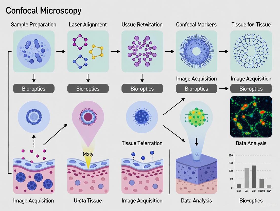
Figure 1: Confocal microscopy workflow for 3D tissue imaging, highlighting critical setup steps.
Experimental Protocols
Protocol: Optimizing Confocal Imaging for Skin Permeation Studies
This protocol, adapted from recent methodological improvements, is designed for analyzing drug retention and distribution within skin samples using confocal Raman microscopy or fluorescence-based confocal imaging [4].
4.1.1 Materials and Reagents
- Tissue Samples: Porcine or human skin sections from ex vivo Franz cell diffusion studies.
- Mounting Medium: Phosphate-buffered saline (PBS) or compatible aqueous mounting medium.
- Spacers: Fishing line or coverslip fragments to prevent sample compression.
- Antifading Agents: If required for prolonged imaging of fluorescent samples.
4.1.2 Pre-Measurement Protocol to Mitigate Fluorescence and Shrinkage Laser interactions with skin can cause thermal damage, fluorescence, and sample shrinkage, particularly under 532 nm excitation. The following pre-measurement steps are recommended:
- Laser-Induced Photobleaching: Perform three consecutive Raman (or fluorescence) mapping measurements (XY scans) over the same region with gradually increasing laser exposure.
- Progressive Illumination: This series of pre-scans serves to photobleach endogenous fluorophores, thereby reducing background fluorescence and stabilizing the sample for subsequent quantitative analysis.
- Hydration Control: Maintain elevated hydration levels consistent with diffusion studies, but be aware that this is associated with increased laser-induced shrinkage. For dehydrated state analysis, freeze-drying is an option but may lead to unpredictable sample movement and reduced spectral quality at depth [4].
4.1.3 Image Acquisition and Analysis
- Spatial Distribution Assessment: Acquire images using both XY mapping at successive depths (Z-stack) and imaging of physical skin cross-sections.
- Quantitative Analysis: Analyze the distribution of your compound of interest (e.g., 4-cyanophenol). The protocol should reveal reduced compound content with increasing skin depth and higher concentration correlated with longer exposure times during diffusion studies [4].
Protocol: General Specimen Preparation for High-Resolution Confocal Imaging of Tissues
Proper specimen preparation is paramount for achieving high-quality confocal images and is often the most critical factor for success [3].
4.2.1 Fixation and Staining
- Fixation: Begin with a standard fixation protocol known to be effective for your tissue type and antigen of interest in conventional fluorescence microscopy. Common fixatives include 4% paraformaldehyde.
- Staining: For immunofluorescence, use fluorochromes matched to your microscope's laser lines. Note that due to optical sectioning, samples may require increased staining times or stain concentrations for confocal analysis compared to wide-field microscopy, as the confocal microscope undersamples fluorescence in thick specimens [3].
4.2.2 Mounting
- Preserve 3D Structure: To maintain the three-dimensional structure of the tissue, use a spacer between the slide and coverslip to avoid crushing the specimen.
- Mounting Medium: Use an anti-fade mounting medium appropriate for your fluorophores. Match the refractive index of the mounting medium to that of the objective lens immersion medium (e.g., oil, glycerol) for optimal resolution [3].
4.2.3 Microscope Setup and Imaging
- Objective Lens Selection: Choose a high numerical aperture (NA) objective lens. A higher NA provides better resolution, a thinner optical section, and collects more light, resulting in a brighter image [3].
- Pinhole Adjustment: Set the pinhole diameter to 1 Airy Unit (AU) as a starting point for the optimal balance between section thickness and signal strength. Adjust as needed based on signal intensity and desired section thickness (refer to Table 1).
- Laser Power and Detector Gain: Use the minimal laser power necessary to obtain a good signal to minimize photobleaching and phototoxicity. Set the detector gain to avoid signal saturation ("clipped" pixels), which destroys quantitative information [3] [5].
- Z-Stack Acquisition: Define the top and bottom of your region of interest and acquire sequential optical sections at intervals no greater than half the axial resolution of your objective (as defined by the Nyquist criterion) for accurate 3D reconstruction.
The Scientist's Toolkit: Essential Materials for Confocal Imaging
Successful confocal imaging requires careful selection of reagents and materials. The following table details key solutions and their functions in the context of tissue preparation and imaging.
Table 3: Research Reagent Solutions for Confocal Microscopy
| Item Name | Function & Application | Example/Note |
|---|---|---|
| High-NA Immersion Objective | Focuses laser light and collects emitted signal; determines resolution and light-gathering capability. | 60x oil immersion, NA 1.4 for highest resolution of subcellular details [3]. |
| Cyanine Dyes (Cy3, Cy5) | Synthetic fluorophores for immunofluorescence; often brighter and more photostable than traditional dyes. | Cy3 is a rhodamine alternative; Cy5 is useful for triple-labeling due to its far-red emission [3]. |
| Antifade Mounting Medium | Preserves fluorescence by reducing photobleaching during imaging, crucial for multi-channel or 3D acquisition. | Commercial formulations like ProLong Diamond or VECTASHIELD [3]. |
| Phosphate Buffered Saline (PBS) | A physiological pH buffer used for washing samples, diluting antibodies, and as a base for mounting media. | Standard 0.1 M concentration, pH 7.4, is used in specimen preparation protocols [6]. |
| Glutaraldehyde | A cross-linking fixative that provides excellent preservation of ultrastructure for EM and some confocal applications. | Often used in combination with other fixatives; 2.5% solution for cell pellets [6]. |
The core principles of confocal microscopy—optical sectioning and the resultant signal-to-noise advantage—make it an indispensable tool for modern tissue research and drug development. By physically rejecting out-of-focus light, confocal systems provide the high-contrast, high-resolution data necessary to analyze the three-dimensional architecture of tissues and the subcellular localization of biomolecules. Adherence to optimized protocols for sample preparation, microscope setup, and image acquisition is critical for leveraging the full potential of this technology. As innovations such as photon-counting detectors [5] and improved NIR dyes continue to emerge, the capabilities of confocal microscopy for deep-tissue, quantitative analysis will only expand, further solidifying its role as a cornerstone of biomedical imaging.
In the realm of biological research, confocal microscopy has revolutionized our ability to visualize tissue architecture and molecular composition with high resolution and three-dimensional clarity. The fidelity of this imaging, however, is profoundly dependent on the preceding steps of sample preparation, from tissue sectioning to antibody staining. This application note provides a consolidated guide to the essential reagents and equipment required for successful confocal microscopy of tissue samples, framing them within detailed, executable protocols. The information is tailored for researchers, scientists, and drug development professionals aiming to generate reproducible, high-quality data for their research theses and projects.
The Scientist's Toolkit: Core Equipment and Reagents
A successful confocal microscopy experiment is built on a foundation of specific equipment and high-quality reagents. The following table catalogues the essential items and their critical functions in the workflow.
Table 1: Essential Research Reagent Solutions and Equipment for Confocal Microscopy
| Item | Function/Application | Specific Examples |
|---|---|---|
| Cryostat | Sectioning fixed or fresh-frozen tissues into thin slices (e.g., 4-5 µm) for microscopy. [7] [8] | Leica CM1950 [8] |
| Microtome | Sectioning paraffin-embedded tissues. [8] | Leica RM 2135 [8] |
| Confocal Microscope | High-resolution imaging with optical sectioning capability to minimize out-of-focus light. [9] | Olympus FV1000 [7], Nikon C2 [10], Leica Stellaris 5 [9] |
| Primary Antibodies | Specific binding to target antigens (e.g., MyHC isoforms, endothelial markers). [7] [9] [10] | Anti-αSMA (Sigma-Aldrich) [7], Anti-MyHC clones (BA-F8, SC-71) [9], Anti-CD31 (Millipore) [10] |
| Secondary Antibodies | Fluorophore-conjugated antibodies that bind to primaries for detection. [8] [9] | Goat anti-mouse IgG1 (Alexa Fluor 488) [9] |
| Fluorophores | Fluorescent dyes excited by laser light for detection. [9] | Alexa Fluor 488, 546, 647, 750 [9] |
| Mounting Medium | Preserves samples and often contains counterstains like DAPI for nuclei. [8] [9] | Aqueous Fluoroshield with DAPI [8], SlowFade Diamond [9], Fluoromount-G [10] |
| Tissue Freezing Medium | Supports tissue structure for cryosectioning. [8] | Leica Tissue Freezing Medium [8] |
| Blocking Buffer | Reduces nonspecific antibody binding. [10] | 3% BSA, 5% Donkey Serum, 0.1% Triton X-100 in PBS [10] |
Detailed Experimental Protocols
Protocol 1: Cryosectioning of Spheroid and Tissue Samples
This protocol is adapted for handling both soft 3D spheroid models and larger tissue samples, ensuring the preservation of morphology for subsequent staining. [8]
Workflow Overview:
Materials:
- Equipment: Cryostat (e.g., Leica CM1950) [8], micropipettes, microcentrifuge tubes.
- Reagents: 4% Formaldehyde in PBS (pH 7.2-7.4), Phosphate-Buffered Saline (PBS), 30% Sucrose in PBS, Tissue Freezing Medium (e.g., from Leica) [8].
Step-by-Step Methodology:
- Transfer and Collection: Use a micropipette with a tip or a plastic Pasteur pipette to transfer spheroids from culture plates into a microcentrifuge tube containing cold 4% formaldehyde. Visually confirm the spheroid is within the tip before dispensing. For tissues, proceed to fixation. [8]
- Fixation: Submerge the samples in cold 4% formaldehyde for 15 minutes at room temperature to preserve structure. [8]
- Washing: Remove the fixative and wash the samples three times in PBS for 5 minutes each to remove residual fixative. [8]
- Cryoprotection: Remove PBS and submerge the samples in 30% sucrose in PBS for at least 2 hours at room temperature or overnight at 4°C. This step prevents ice crystal formation during freezing. [8]
- Embedding: a. Apply a small amount of tissue freezing medium to a cryostat specimen disk. b. Place it in the cryostat for 1-2 minutes to partially harden. c. Using a scalpel, transfer the spheroid or tissue onto the semi-solid medium. d. Return the disk to the cryostat to complete hardening. [8]
- Cryosectioning: Cut sections at a thickness of 5 µm using the cryostat and mount them onto microscope slides. [8]
- Storage: Store slides at -20°C or -80°C until ready for staining.
Protocol 2: Immunofluorescence Staining for Confocal Microscopy
This protocol details the steps for fluorescently labeling tissue sections or whole-mount tissues for high-resolution imaging, using an anterior eye cup whole-mount as an example. [10]
Workflow Overview:
Materials:
- Equipment: Confocal microscope (e.g., Nikon C2), humidified chamber, fine-tip forceps. [10]
- Reagents: Fixative (4% Formaldehyde), PBST (0.1% Triton X-100 in PBS), Blocking Buffer (3% BSA, 5% Donkey Serum, 0.1% Triton X-100), primary and secondary antibodies, mounting medium with DAPI (e.g., Fluoromount-G) [10].
Step-by-Step Methodology:
- Tissue Harvest and Fixation: Euthanize the animal according to approved institutional protocols. Harvest the tissue of interest (e.g., eyeball) and fix it in 4% formaldehyde for 50 minutes at room temperature with gentle shaking. For whole-mount tissues, a small incision can be made to mark orientation. [10]
- Permeabilization and Blocking: Incubate the tissue in PBST to permeabilize cell membranes. Then, incubate in blocking buffer for a minimum of 2 hours or overnight at 4°C to block nonspecific binding sites. [10]
- Primary Antibody Incubation: Incubate the tissue with the primary antibody diluted in blocking buffer. For whole-mount tissues, this typically requires 2-3 days at 4°C with gentle agitation to ensure sufficient penetration. [10]
- Washing: Wash the tissue extensively with PBST, with changes every few hours, over a period of 1-2 days to remove unbound primary antibody. [10]
- Secondary Antibody Incubation: Incubate the tissue with fluorophore-conjugated secondary antibodies (e.g., Alexa Fluor dyes) diluted in blocking buffer, protected from light, for 1-2 days at 4°C. [10]
- Final Washing: Perform a final series of washes with PBST, as in step 4, to remove unbound secondary antibody. [10]
- Mounting: Mount the tissue on a microscope slide using an appropriate mounting medium containing DAPI to counterstain nuclei. Carefully place a coverslip and seal the edges. [10]
Protocol 3: Image Acquisition and Analysis on a Confocal Microscope
This protocol outlines the process of acquiring high-quality, publication-ready images from prepared samples.
Workflow Overview:
Materials:
- Equipment: Advanced confocal microscope system (e.g., Leica Stellaris 5 with white light laser) [9].
- Software: Microscope operating software (e.g., NIS-Elements, Fluoview FV10-ASW), ImageJ/Fiji, Imaris. [7] [10]
Step-by-Step Methodology:
- Microscope Setup: Turn on the microscope, lasers, and associated computer system. Place the prepared slide on the stage.
- Laser and Detector Setup: Select the appropriate laser lines for the fluorophores used (e.g., 405 nm for DAPI, 488 nm for Alexa Fluor 488). Set detection bandwidths (or use spectral detectors) to minimize bleed-through between channels. For systems with white light lasers (WLL), fine-tune excitation wavelengths for optimal spectral unmixing. [9]
- Z-Stack Acquisition: To capture 3D information, set the upper and lower limits of the sample region and define the number of optical sections (step size). The "extended z-length" feature on some systems ensures complete imaging of all focal planes, accounting for tissue unevenness. [9]
- Spectral Unmixing: If multiple fluorophores with overlapping spectra are used, employ the microscope's spectral unmixing functionality. This uses reference spectra to mathematically separate the signals, reducing bleed-through and improving signal clarity. [9]
- Image Processing and Analysis: Use software like ImageJ or Imaris for post-processing tasks. This can include maximum intensity projection of Z-stacks, 3D reconstruction, quantification of fluorescence intensity, measurement of fiber cross-sectional areas, and co-localization analysis. [9] [10]
Advanced Applications and Future Directions
The principles outlined here form the basis for more complex applications. For instance, in intraoperative cancer diagnosis, confocal microscopy (e.g., Histolog Scanner) can image fresh lumpectomy specimens after staining with a fluorescent dye (acridine orange), providing pathological feedback on margin status within minutes with high accuracy (95.2% in one study). [11] Furthermore, technological advancements continue to push boundaries. Techniques like Confocal² Spinning-Disk Image Scanning Microscopy (C2SD-ISM) combine physical out-of-focus rejection with computational super-resolution, achieving lateral resolutions of 144 nm and enabling high-fidelity imaging at depths of up to 180 µm in tissues. [12] For drug development, confocal Raman microscopy offers a label-free method to analyze the spatial distribution of drugs within tissues, such as skin, though it requires careful pre-measurement protocols to mitigate issues like laser-induced fluorescence and sample damage. [4]
Mastering the confocal microscopy workflow—from the precise execution of cryosectioning and immunostaining to the optimized operation of the microscope itself—is fundamental to modern tissue-based research. The essential reagents and equipment detailed in this application note, when applied within the framework of robust and reproducible protocols, empower scientists to generate high-quality, quantifiable data. This rigorous approach to sample preparation and image acquisition is indispensable for validating hypotheses in academic theses and for driving innovation in preclinical drug development.
Tissue Harvesting, Fixation, and Cryopreservation Best Practices
For research utilizing confocal microscopy, the quality of the final image is fundamentally determined by the initial steps of tissue preparation. Proper harvesting, fixation, and cryopreservation are critical to preserving tissue architecture, cellular ultrastructure, and biomolecule integrity. Suboptimal protocols introduce artifacts, degrade fluorescence signals, and compromise the validity of microscopic data. This application note provides detailed, current methodologies to prepare tissue samples for high-resolution confocal microscopy, ensuring that the observed structures accurately represent the living state. Adherence to these protocols maintains antigenicity for immunostaining, minimizes autofluorescence, and ensures the structural integrity necessary for three-dimensional reconstruction in deep-tissue imaging.
Tissue Harvesting and Initial Processing
The immediate post-harvest period is a critical window where rapid action prevents degradation and preserves in vivo conditions.
Core Principles and Procedures
- Rapid Processing: Minimize the ischemic time as much as possible. The time between tissue excision and fixation/cooling should be documented and kept consistent across samples to reduce variability [13].
- Aseptic Technique: Perform dissection in a sterile environment using sterilized instruments to prevent microbial contamination that can degrade tissue and generate background fluorescence.
- Tissue Size Considerations: For subsequent fixation and cryopreservation, ideal tissue blocks should not exceed 5 mm x 5 mm x 3 mm. This size allows for rapid and uniform penetration of fixatives and cryoprotectants, which is vital for preserving deep-tissue structures for confocal analysis [14].
- Physiological Buffers: During dissection, keep tissues moist with ice-cold, oxygenated physiological buffers (e.g., PBS or Hank's Balanced Salt Solution) to prevent dehydration and cold ischemia.
Sample Labeling and Documentation
Label all samples comprehensively with unique identifiers. Record critical metadata including donor/sample ID, date and time of harvest, tissue type, and preservation method. Consistent labeling and record-keeping are foundational to reproducible research [13].
Fixation Strategies for Confocal Microscopy
Fixation stabilizes tissue morphology by cross-linking proteins and nucleic acids, preventing decay and preparing samples for staining and imaging.
Chemical Fixation: Formalin-Fixed Paraffin-Embedded (FFPE)
The FFPE method is a cornerstone for histological analysis and provides excellent morphological preservation.
- Protocol: Immerse tissue in 10% neutral buffered formalin for 18-24 hours at room temperature. Under-fixation compromises structural integrity, while over-fixation can mask antigen epitopes, hindering antibody binding for immunofluorescence. Following fixation, dehydrate the tissue through a graded series of ethanol, clear with xylene, and infiltrate and embed with paraffin wax [13].
- Advantages for Imaging: FFPE blocks can be stored indefinitely at 4°C and sectioned thinly, facilitating high-resolution 2D imaging. The process is well-standardized, yielding consistent samples for comparative studies [13].
- Disadvantages for Confocal Microscopy: The embedding process can introduce autofluorescence. Furthermore, antigen retrieval steps are often required to unmask epitopes for antibody labeling, which can be harsh and may damage some targets.
Chemical Fixation for Fluorescence Imaging
For samples destined primarily for fluorescence confocal microscopy, paraformaldehyde (PFA) perfusion is the gold standard.
- Protocol: For the most pristine preservation, perform transcardial perfusion with ice-cold 4% PFA in phosphate buffer. This delivers the fixative rapidly and uniformly throughout the vasculature, immobilizing antigens in their native locations. Post-perfusion, dissect the tissue of interest and post-fix by immersion in 4% PFA for 4-6 hours at 4°C to complete the fixation process [15]. Prolonged immersion fixation should be avoided to reduce autofluorescence.
- Application: This method is particularly suited for delicate tissues like brain, where synaptic structures and neural pathways must be preserved for 3D reconstruction using tissue clearing techniques [15].
Table 1: Comparison of Primary Fixation Methods for Confocal Microscopy
| Parameter | Formalin-Fixed Paraffin-Embedded (FFPE) | Perfusion/Immersion with Paraformaldehyde (PFA) |
|---|---|---|
| Primary Use | Long-term archival, histopathology, 2D imaging | Immunofluorescence, 3D imaging, tissue clearing |
| Tissue Morphology | Excellent | Excellent |
| Antigen Preservation | Variable; often requires retrieval | Superior; less epitope masking |
| Autofluorescence | Moderate (can be introduced by processing) | Low (if protocol is optimized) |
| Compatibility with Deep-Tissue Imaging | Low (requires sectioning) | High (suitable for whole-mounts) |
| Storage | Indefinite at 4°C [13] | Several months to years at 4°C |
Cryopreservation and Long-Term Storage
Cryopreservation halts biological activity, preserving tissues in a state of suspended animation for long-term storage while maintaining protein function and viability.
Snap-Freezing
This method is used when immediate halting of enzymatic activity is required for biochemical assays.
- Protocol: Embed the tissue in Optimal Cutting Temperature (OCT) compound and rapidly submerge it in a slurry of isopentane pre-cooled by liquid nitrogen, or directly into liquid nitrogen. Rapid cooling minimizes the formation of damaging ice crystals. Store snap-frozen samples at -80°C [13].
Cryopreservation with Cryoprotectants
For preserving cellular viability and structure for applications like live-cell imaging or cell culture, controlled freezing with cryoprotectants (CPAs) is essential.
- Principle: CPAs like Dimethyl Sulfoxide (DMSO) and glycerol protect cells by reducing ice crystal formation and mitigating osmotic shock during freezing and thawing [16].
- General Protocol: Gradually equilibrate tissue with a CPA solution (e.g., 10% DMSO in culture medium). Use a controlled-rate freezer to slowly cool the sample to approximately -80°C at a rate of 1°C per minute before transferring to long-term storage in liquid nitrogen (-196°C) [16].
- Vitrification: For especially sensitive tissues like ovarian tissue, vitrification—an ice-free preservation method using high CPA concentrations and ultra-rapid cooling—is employed. This technique shows promise for minimizing cryo-injuries that can distort tissue architecture [17] [14].
Table 2: Thermophysical Properties of a Representative Cryopreservation Medium for Ovarian Tissue [18]
| Property | Value | Protocol Implication |
|---|---|---|
| Glass Transition Temperature (Tg') | -120.49 °C | Safe long-term storage temperature |
| Crystallization Temperature (Tc) | -20 °C (at 2.5 °C/min) | Temperature at which ice forms during cooling |
| Melting Temperature (Tm) | -4.11 °C | Temperature at which ice melts during warming |
Thawing Protocols
Thawing is as critical as freezing. Rapid thawing is generally recommended to avoid ice recrystallization.
- Optimized Protocol: As demonstrated for ovarian tissue, a two-step thawing process can be highly effective. This involves a slow initial warming in a cold chamber to reach the glass transition temperature (Tg'), followed by a rapid incubation at 37°C to quickly pass the melting point (Tm), thereby limiting thermal and mechanical shocks [18].
Experimental Protocols for Validation via Confocal Microscopy
After processing, validation of tissue quality through staining and imaging is a crucial final step.
Immunolabeling of Thick Tissue Sections
This protocol is adapted for staining vibratome sections or cleared tissues for deep imaging.
- Materials:
- Primary Antibody: Specific to the target antigen (e.g., Anti-CD31 for vasculature [15]).
- Secondary Antibody: Fluorophore-conjugated, species-specific (e.g., Alexa Fluor 488 [15]).
- Permeabilization/Blocking Solution: PBS with 0.2% Triton X-100, 10% DMSO, and 6% Donkey Serum [15].
- Washing Buffer: PBS with 0.2% Tween-20 and 10 μg/ml heparin (PTwH) [15].
- Methodology:
- Permeabilization and Blocking: Incubate tissues in permeabilization/blocking solution at 37°C for 1-3 days to ensure antibody penetration and reduce non-specific binding.
- Primary Antibody Incubation: Incubate with primary antibody diluted in PTwH with 5% DMSO and 3% serum at 37°C for 3-4 days.
- Washing: Wash the tissue extensively with PTwH for 24 hours to remove unbound antibody.
- Secondary Antibody Incubation: Incubate with fluorophore-conjugated secondary antibody in PTwH with 3% serum at 37°C for 2-3 days, protected from light.
- Final Wash: Perform a final wash in PTwH before proceeding to imaging or tissue clearing [15].
Live-Cell Imaging in 3D Cultures
For imaging live cells within a 3D scaffold, specific precautions are necessary.
- Materials: Alvetex Scaffold, HEPES-buffered imaging medium, vital fluorescent dyes (e.g., CellTracker CM-DiI, Hoechst 33342) [19].
- Methodology:
- Staining: For hydrophobic dyes like DiI, stain cells in suspension prior to seeding into the 3D scaffold to prevent non-specific binding to the scaffold material.
- Microscope Setup: Use a confocal microscope with a temperature-controlled stage (37°C) and CO₂ supply. Equilibrate the stage insert overnight to prevent focal drift.
- Imaging Parameters: To minimize photobleaching and light toxicity, use low laser power, short exposure times, and ensure shutters are closed between acquisitions. The imaging depth in a 200 μm scaffold may be limited to 50-100 μm [19].
The Scientist's Toolkit: Essential Reagents and Materials
Table 3: Key Research Reagent Solutions for Tissue Processing and Imaging
| Reagent/Material | Function | Example Application |
|---|---|---|
| Paraformaldehyde (PFA) | Protein cross-linking fixative | Preserving cellular ultrastructure for immunofluorescence [15] |
| Cryoprotectants (DMSO, Glycerol) | Reduce ice crystal formation during freezing | Maintaining cell viability in cryopreserved tissues [16] |
| Alvetex Scaffold | Polystyrene scaffold for 3D cell culture | Creating in-vivo-like environments for live-cell imaging [19] |
| Triton X-100 & Tween-20 | Detergents for membrane permeabilization and washing | Enabling antibody penetration during immunolabeling [15] |
| Donkey Serum | Protein source for blocking non-specific binding | Reducing background fluorescence in immunoassays [15] |
| HEPES-buffered Medium | Maintains physiological pH without CO₂ | Live-cell imaging on microscopes without a CO₂ supply [19] |
| Sucrose | Non-penetrating cryoprotectant and osmotic buffer | Osmotic protection in vitrification solutions [14] [18] |
Mastering the integrated pipeline of tissue harvesting, fixation, and cryopreservation is a prerequisite for generating reliable, high-quality data in confocal microscopy. The protocols detailed herein—from the speed of harvest to the precision of thawing—are designed to safeguard the native state of tissues against the artifacts introduced by poor handling. By adhering to these best practices and leveraging the outlined reagent toolkit, researchers can confidently prepare samples that are optimally preserved for the demands of modern, high-resolution bioimaging, thereby ensuring that their microscopic observations are a true reflection of biological reality.
In confocal microscopy, the careful selection of fluorescent probes is a cornerstone of experimental success, particularly when investigating complex tissue samples. Biological laser scanning confocal microscopy relies heavily on fluorescence due to the high degree of sensitivity afforded by the technique and its ability to specifically target structural components and dynamic processes in both fixed and living specimens [20]. The selection of appropriate fluorophores directly impacts data quality, influencing signal-to-noise ratios, resolution of subcellular structures, and the accuracy of multi-color experiments. This application note provides a structured framework for selecting fluorophores based on critical parameters—brightness, photostability, and spectral profile—within the context of confocal microscopy protocols for tissue research, ensuring reliable and interpretable results for researchers, scientists, and drug development professionals.
Fundamental Fluorophore Properties
Key Characteristics for Selection
Fluorophores are characterized by several quantifiable properties that determine their performance in imaging applications. Understanding these parameters is essential for making an informed selection.
- Brightness: The practical brightness of a fluorophore is a function of its molar extinction coefficient (ε) and its fluorescence quantum yield (QY) [20] [21]. The extinction coefficient is a direct measure of a molecule's ability to absorb light, while the quantum yield represents the efficiency with which absorbed photons are converted into emitted photons. A high quantum yield (close to 1.0) is generally desirable [20].
- Photostability: This refers to a fluorophore's resistance to photobleaching, the irreversible degradation of its ability to fluoresce under prolonged or intense illumination [22]. In confocal microscopy, where focused laser beams create high power densities, photostability is critical for acquiring multi-frame time-series or Z-stacks without significant signal loss [20].
- Spectral Profiles: The absorption (excitation) and emission spectra define the light wavelengths a fluorophore uses. The Stokes shift is the difference (in nanometers) between the peak excitation and peak emission wavelengths [21]. A larger Stokes shift can help minimize self-reabsorption and simplify the separation of excitation light from emitted fluorescence.
Quantifying Fluorophore Characteristics
The following table summarizes the key quantitative parameters for fluorophore evaluation.
Table 1: Key Quantitative Parameters for Fluorophore Evaluation
| Parameter | Definition | Significance in Confocal Microscopy |
|---|---|---|
| Molar Extinction Coefficient (ε) | Measure of the ability to absorb light at a specific wavelength [20] [21]. | A higher ε value indicates greater light absorption per fluorophore, contributing to a brighter signal. |
| Quantum Yield (QY) | Ratio of photons emitted to photons absorbed [20] [21]. | A higher QY (max 1.0) indicates more efficient photon emission. Directly contributes to brightness. |
| Brightness | Product of ε and QY [21]. | The overall intrinsic signal intensity of the fluorophore. A primary criterion for selection. |
| Stokes Shift | Difference between peak excitation and emission wavelengths [21]. | A larger shift reduces spectral overlap, simplifying filter selection and reducing background. |
| Photobleaching Rate | The rate constant of irreversible fluorescence loss under illumination [22]. | A slower rate is vital for time-lapse imaging and for collecting 3D image stacks. |
Spectral Selection and Multi-Color Imaging
The Challenge of Spectral Bleed-Through
A primary challenge in multi-color fluorescence microscopy is spectral bleed-through (also called crossover or crosstalk). This artifact occurs when the emission of one fluorophore is detected in the photomultiplier channel reserved for another [23] [24]. This is largely due to the broad and asymmetrical emission profiles of many fluorophores, which often have long "tails" extending into longer wavelengths [23] [25]. Bleed-through can lead to the misinterpretation of results, particularly in co-localization studies or quantitative measurements like FRET [23].
Laser Compatibility
Confocal microscopy excites fluorophores using specific laser spectral lines, which are only a few nanometers wide [20]. Therefore, a fluorophore must have strong absorption at a available laser line to be effective. The table below lists common laser lines and examples of compatible fluorophores.
Table 2: Common Confocal Laser Lines and Compatible Fluorophores
| Laser Type | Spectral Line (nm) | Example Fluorophores |
|---|---|---|
| Diode | 405 | mTagBFP2 [26] |
| Diode | 440 | |
| Argon-Ion | 488 | Fluorescein (FITC), Alexa Fluor 488, EGFP [20] [26] |
| DPSS | 561 | Alexa Fluor 546, mCherry, mApple [20] [26] |
| He-Neon | 633 | Alexa Fluor 633, Cy5 [20] |
| Diode | 640 | Alexa Fluor 647, TagRFP657 [20] [26] |
Practical Selection Protocol for Tissue Samples
A Step-by-Step Guide
This protocol provides a systematic workflow for selecting fluorophores for multi-color confocal imaging of tissue samples, balancing theoretical spectral properties with practical instrumentation constraints.
Step 1: Define Experimental Parameters. Identify the number and type of cellular targets to be labeled. Simultaneously, confirm the specific laser lines and available detection channels (filter sets and spectral ranges) on your confocal microscope [20]. This step aligns biological needs with instrumental capabilities.
Step 2: Select Candidate Fluorophores. Choose fluorophores with high brightness (ε × QY) and whose emission maxima are as far apart as possible [23] [25]. For example, a combination of Alexa Fluor 488 and Alexa Fluor 633 exhibits minimal spectral overlap and is an excellent choice for two-color imaging [23]. Reserve the brightest and most photostable fluorophores for the least abundant targets [23].
Step 3: Assign Fluorophores to Microscope Channels. Configure your microscope's detection channels to minimize bleed-through. Set narrow emission bandpasses around the peak emission of each fluorophore. Image the reddest (longest wavelength) fluorophore first, as its excitation is less likely to excite bluer dyes [23].
Step 4: Optimize Specimen Labeling and Validate. Balance the labeling intensity of the different probes during specimen preparation so that fluorescence emission intensities are similar [23]. A strongly over-labeled target can bleed into other channels even with good spectral separation. Perform control experiments by labeling samples with a single fluorophore each to empirically quantify and correct for any residual bleed-through [25].
Step 5: Image Acquisition. Use sequential scanning (multitracking), where each laser line excites a single fluorophore at a time (line-by-line or frame-by-frame), to virtually eliminate cross-excitation [23] [25]. For highly overlapping probes like some fluorescent protein pairs, employ spectral imaging and linear unmixing, a technique that captures the full emission spectrum per pixel and computationally separates the contributions of each fluorophore based on their unique "fingerprint" [25] [24].
Advanced Application: FRET Fluorophore Selection
Förster Resonance Energy Transfer (FRET) is a mechanism describing energy transfer between two light-sensitive molecules, a donor and an acceptor, when they are in close proximity (typically 1-10 nm) [27] [28]. FRET efficiency is extremely sensitive to distance, making it a powerful tool for studying protein-protein interactions and conformational changes [27].
Key Criteria for FRET Pairs
Selecting an optimal donor-acceptor pair is critical for a successful FRET experiment.
- Spectral Overlap: There must be a significant overlap between the donor's emission spectrum and the acceptor's absorption spectrum [27] [28]. This overlap is quantified by the spectral overlap integral (J).
- Förster Radius (R₀): This is the distance at which FRET efficiency is 50%. A larger R₀ indicates a more sensitive FRET pair. R₀ depends on the quantum yield of the donor, the extinction coefficient of the acceptor, the spectral overlap, and the relative orientation of the dipoles (κ²) [27] [28].
- Donor-Acceptor Proximity: The donor and acceptor must be within a range of ~0.5 R₀ to 1.5 R₀ for measurable FRET to occur [28].
Table 3: Essential Criteria for Selecting a FRET Donor-Acceptor Pair
| Criterion | Requirement | Rationale |
|---|---|---|
| Spectral Overlap | High overlap between donor emission and acceptor absorption [27] [28]. | Prerequisite for dipole-dipole coupling and energy transfer. |
| Donor Quantum Yield | High. | Increases the Förster radius (R₀), making the pair more sensitive to distance changes [28]. |
| Acceptor Extinction Coefficient | High. | Increases the Förster radius (R₀) [28]. |
| Minimal Direct Acceptor Excitation | Acceptor should not be significantly excited at the donor's excitation wavelength. | Reduces background and false-positive FRET signals. |
| Fluorescent Protein Folding | Efficient folding and maturation at physiological conditions. | Critical for live-cell FRET experiments using genetically encoded biosensors [28]. |
FRET Experimental Workflow
A generalized protocol for a sensitized emission FRET experiment is outlined below.
- Construct Design: Genetically fuse the donor and acceptor fluorescent proteins (e.g., CFP/YFP or newer variants like mCerulean3/mVenus) to the proteins of interest [28] [26]. Ensure the linker allows for proper folding and freedom of movement.
- Microscope Setup: Configure the microscope with three filter sets:
- Donor channel: Donor excitation / donor emission.
- Acceptor channel: Acceptor excitation / acceptor emission.
- FRET channel: Donor excitation / acceptor emission.
- Image Acquisition: Acquire images of the specimen in all three channels using sequential scanning to prevent bleed-through.
- FRET Efficiency Calculation: Calculate the FRET efficiency using the formula: ( E = 1 - \tau{D}' / \tau{D} ), where ( \tau{D}' ) and ( \tau{D} ) are the donor fluorescence lifetimes in the presence and absence of the acceptor, respectively [27]. Alternatively, for intensity-based measurements, efficiency can be calculated from the sensitized acceptor emission after careful correction for spectral bleed-through [28].
The Scientist's Toolkit: Research Reagent Solutions
The following table catalogs essential materials and resources used in fluorescence imaging for tissue research.
Table 4: Essential Research Reagents and Tools for Fluorescence Imaging
| Reagent / Tool | Function and Utility |
|---|---|
| Synthetic Fluorophores (e.g., Alexa Fluor dyes) | Bright, photostable dyes with a range of excitation/emission profiles. Often conjugated to antibodies (immunofluorescence) or phalloidin (F-actin staining) for specific labeling of cellular structures in fixed tissues [20] [23]. |
| Fluorescent Proteins (e.g., GFP, mCherry variants) | Genetically encoded tags for live-cell imaging, allowing tracking of protein localization, dynamics, and expression in real time [28] [25] [26]. |
| Organelle-Specific Probes (e.g., MitoTrackers) | Cell-permeant fluorescent dyes that selectively accumulate in specific organelles (e.g., mitochondria, lysosomes), enabling study of organelle morphology and function in live or fixed cells [21]. |
| Spectral Viewers (Online Tools) | Software tools provided by microscope and reagent manufacturers that allow visualization of fluorophore spectra. They are crucial for predicting laser compatibility and potential spectral overlap during experimental design [21]. |
| Spectral Imaging & Linear Unmixing Software | Advanced microscope hardware and software solutions that capture the full emission spectrum per pixel and computationally separate the signals of multiple, spectrally overlapping fluorophores [25] [24]. |
Step-by-Step Staining, Imaging, and 3D Analysis Protocol
Optimized Immunostaining Protocol for Multiplexed Fiber Typing (e.g., MyHC isoforms)
Within the context of confocal microscopy research for tissue samples, the precise identification of muscle fiber types through their respective myosin heavy chain (MyHC) isoforms is a fundamental technique in muscle physiology and pathology studies [9]. Muscle fibers are historically categorized based on the expression of specific MyHC isoforms: Type 1 (slow-twitch), 2A (fast-twitch oxidative), 2X (fast-twitch), and 2B (fast-twitch glycolytic) [9]. The masseter muscle, a key orofacial muscle, demonstrates unique anatomical and functional properties, including sexual dimorphism in MyHC expression and complex fiber architecture, making it a particularly relevant but challenging subject for phenotypic characterization [9].
Conventional fluorescence microscopy has been a cornerstone in muscle fiber typing; however, confocal microscopy offers significant complementary advantages [9]. These include enhanced resolution achieved by minimizing out-of-focus light using a pinhole, increased flexibility for multiplexing, and the ability to capture multiple optical planes for three-dimensional reconstruction of imaged tissue [9]. This protocol details an optimized method for quadruple immunostaining of MyHC isoforms in rodent muscle samples, leveraging the capabilities of modern confocal microscopy systems to achieve robust, high-resolution, and quantifiable multiplexed fiber typing.
Materials and Reagents
Research Reagent Solutions
The following table lists essential materials and reagents required for the immunostaining procedure, along with their specific functions in the protocol.
Table 1: Essential Reagents for Multiplexed Immunostaining
| Reagent/Category | Specific Examples & Details | Primary Function in Protocol |
|---|---|---|
| Primary Antibodies | Anti-MyHC slow (BA-F8, supernatant), Anti-MyHC 2A (SC-71, supernatant), Anti-MyHC 2X (6H1, supernatant), Anti-MyHC 2B (BF-F3, supernatant) [9] [29] | Specific recognition and binding to distinct MyHC isoforms for fiber type identification. |
| Secondary Antibodies | Isotype-specific conjugates (e.g., Goat anti-mouse IgG1 Alexa Fluor 488, Goat anti-Mouse IgM Alexa Fluor 546, Goat anti-Mouse IgG2b Alexa Fluor 647) [9] | Amplification of signal; fluorescent labeling for multiplexed detection using distinct channels. |
| Fixative | 2.5% Glutaraldehyde in 0.1 M phosphate buffer [6] | Preserves cellular ultrastructure and tissue morphology by crosslinking proteins. |
| Blocking Agent | Normal Goat Serum or Bovine Serum Albumin (BSA) [9] | Reduces non-specific antibody binding, thereby minimizing background staining. |
| Permeabilization Agent | PBS + 0.1% Triton X-100 [9] | Disrupts cell membranes to allow antibody penetration into cells and tissue sections. |
| Nuclear Counterstain | DAPI (4',6-Diamidino-2-phenylindole) [9] | Fluorescently labels cell nuclei, aiding in the visualization of cellular architecture. |
| Mounting Medium | SlowFade Diamond antifade mountant [9] | Preserves fluorescence and reduces photobleaching during microscopy and storage. |
Equipment
- Confocal Microscope: Preferably equipped with a white light laser (WLL) and spectral detection capabilities for optimal multiplexing and unmixing [9].
- Cryostat for tissue sectioning.
- Humidity chamber for antibody incubation steps [30].
Experimental Protocol
Sample Preparation and Fixation
- Tissue Harvesting and Freezing: Dissect the target muscle (e.g., rodent masseter) and immediately embed the tissue in an Optimal Cutting Temperature (O.C.T.) compound. Snap-freeze the embedded tissue in 2-methylbutane pre-cooled by liquid nitrogen. Store samples at -80°C until sectioning [9].
- Sectioning: Using a cryostat, cut thin sections (recommended 5-10 µm thickness) and mount them onto charged glass slides. Allow slides to air dry thoroughly.
- Fixation: Fix the tissue sections by immersing slides in a solution of 2.5% glutaraldehyde prepared in 0.1 M phosphate buffer (pH 7.4) for a minimum of 2 hours at room temperature [6]. Note: Glutaraldehyde provides superior ultrastructural preservation but may introduce autofluorescence; its concentration and fixation time should be optimized.
- Washing: After fixation, wash the slides five times for 3 minutes each in 0.1 M phosphate buffer (pH 7.4) to remove excess fixative [6].
Immunostaining Procedure
The following workflow outlines the key steps for the multiplexed immunostaining protocol.
Figure 1: Experimental workflow for multiplexed immunostaining, detailing the sequential steps from sample preparation to final imaging.
- Blocking and Permeabilization: Incubate the fixed tissue sections in a blocking solution, such as PBS containing 0.1% Triton X-100 and 5% Normal Goat Serum (or 1-5% BSA), for 1 hour at room temperature. This step blocks non-specific binding sites and permeabilizes the tissue [9] [30].
- Primary Antibody Incubation: Prepare a cocktail of the four primary antibodies (MyHC1, 2A, 2X, 2B) in the blocking solution. Apply the mixture to the tissue sections and incubate in a humidity chamber for a minimum of 2 hours at room temperature or overnight at 4°C for enhanced sensitivity [29].
- Washing: Wash the slides thoroughly with PBS containing 0.1% Triton X-100 (PBS-T) three times, for 5 minutes each, to remove unbound primary antibodies.
- Secondary Antibody Incubation: Prepare a cocktail of the corresponding isotype-specific secondary antibodies, each conjugated to a distinct fluorophore (e.g., Alexa Fluor 488, 546, 647), in the blocking solution. Apply the mixture to the sections and incubate for 1 hour at room temperature, protected from light [9].
- Nuclear Staining and Final Wash: Incubate the sections with DAPI (e.g., 1 µg/mL in PBS) for 5-10 minutes to label nuclei. Perform a final wash in PBS for 5 minutes.
- Mounting: Apply a few drops of an antifade mounting medium (e.g., SlowFade Diamond) to the tissue section and carefully place a coverslip on top, avoiding air bubbles. Seal the edges with clear nail polish if necessary. Allow the mountant to cure before proceeding to imaging.
Confocal Microscopy Imaging Setup
To overcome the limitations of widefield fluorescence microscopy, such as signal bleed-through and limited resolution, the following confocal microscopy setup is recommended [9]:
- Microscope System: Use a confocal microscope system equipped with a white light laser (WLL). WLL allows for fine-tuning of excitation wavelengths, which is crucial for efficient spectral unmixing when using multiple fluorophores with close emission spectra [9].
- Spectral Unmixing: Leverage the system's spectral detection capabilities to create a reference spectrum for each fluorophore used. Apply linear unmixing during or after acquisition to accurately distinguish the signals from the different fluorophores and minimize bleed-through [9].
- Z-Stack Acquisition: For detailed three-dimensional analysis or to account for variations in tissue flatness, acquire images as z-stacks. The z-length can be extended beyond the physical thickness of the sample to ensure complete imaging of all focal planes [9].
- Laser Power and Detector Settings: Optimize laser power and detector gain/offset for each channel to maximize the signal-to-noise ratio while avoiding pixel saturation and minimizing photobleaching.
Data Analysis and Quantification
Following image acquisition, quantitative analysis can be performed to determine fiber type composition and morphology.
- Fiber Segmentation: The high-contrast images generated by confocal microscopy enable robust segmentation of individual muscle fibers. This can be done manually or by employing automated image analysis algorithms [31] [9]. Deep learning-based segmentation algorithms, such as CellViT for nuclear segmentation, can be employed for precise identification and quantification of cellular structures [31].
- Fiber Typing and Quantification: Based on the specific fluorescence signal for each MyHC isoform, classify each segmented fiber into a specific type (1, 2A, 2X, 2B) or identify hybrid fibers co-expressing multiple isoforms [29].
- Morphometric Analysis: Measure key parameters such as the cross-sectional area (CSA) of individual fibers and the location of nuclei relative to the fiber membrane [9].
Table 2: Key Parameters for Quantitative Analysis of Muscle Fiber Typing
| Quantitative Parameter | Description | Application/Insight |
|---|---|---|
| Fiber Type Proportion | Percentage of each fiber type (1, 2A, 2X, 2B) within the total analyzed fiber population. | Assessment of muscle composition; reveals shifts in fiber type due to training, disease, or aging. |
| Hybrid Fiber Incidence | Percentage of fibers expressing two or more MyHC isoforms simultaneously. | Indicator of fiber type transition or plasticity under various physiological or pathological stimuli [29]. |
| Fiber Cross-Sectional Area (CSA) | The cross-sectional area of individual muscle fibers, measured in µm². | Evaluation of fiber hypertrophy or atrophy; can be type-specific. |
| Nuclear Position | Location of nuclei (e.g., central vs. peripheral) within the fiber. | Marker of muscle regeneration, denervation, or specific myopathies. |
The logical relationship between the experimental stages and the quantitative data they produce is summarized below.
Figure 2: Data generation workflow, illustrating the progression from experimental stages to quantifiable datasets for muscle fiber analysis.
Confocal laser scanning microscopy (CLSM) is an indispensable tool in biomedical research, enabling high-resolution, three-dimensional imaging of fluorescently labeled specimens [32]. For researchers working with tissue samples, achieving optimal image quality requires the precise calibration of three interdependent parameters: laser power, detector gain, and pinhole alignment. This protocol details the systematic optimization of these core settings within the context of tissue-based research, providing a standardized approach for generating reproducible, high-fidelity data in drug development and basic research applications.
The fundamental advantage of confocal microscopy lies in its ability to eliminate out-of-focus light through a pinhole aperture, a principle patented by Marvin Minsky in 1957 [32] [33]. This optical sectioning capability is crucial for visualizing structures within thick, scattering tissue samples. However, this benefit is fully realized only when the system is properly configured. Misconfiguration can lead to photodamage, poor signal-to-noise ratio, and compromised resolution, ultimately affecting data interpretation.
Core Principles and Parameter Relationships
In a confocal microscope, a laser beam is focused onto a diffraction-limited spot within the sample, and the emitted fluorescence is detected through a pinhole aperture that rejects light from outside the focal plane [32] [33]. This process occurs point-by-point to build a digital image. The key parameters controlling this process are intrinsically linked: increasing laser power boosts the fluorescence signal but risks photobleaching and sample damage; raising detector gain amplifies the signal but also increases background noise; and adjusting the pinhole diameter directly controls section thickness and spatial resolution.
Quantitative Performance Metrics
The following table summarizes the key trade-offs and quantitative relationships between the core adjustable parameters and their impact on image quality in tissue imaging.
Table 1: Key Parameter Interactions and Their Impact on Image Quality
| Parameter | Primary Effect | Impact on Resolution | Impact on Signal-to-Noise Ratio | Risk to Sample Viability |
|---|---|---|---|---|
| Laser Power | Increases fluorescence emission signal | Minimal direct impact | Increases initially, then plateaus due to background and bleaching | High (Photobleaching & Phototoxicity) |
| Detector Gain (PMT) | Amplifies detected signal (both signal and noise) | None | Increases to a point, then decreases due to amplified noise | Low |
| Pinhole Size | Controls volume of detected light (optical section thickness) | Significant (Lateral & Axial) [33] | Increases with size, but out-of-focus light also increases | Medium (Increased light dose if opened) |
| Pinhole Alignment | Maximizes signal through pinhole | Critical for achieving theoretical resolution [32] | Dramatic improvement when correctly aligned | Low |
The theoretical resolution limits of a confocal microscope are determined by the excitation wavelength, the numerical aperture (NA) of the objective lens, and the refractive index of the mounting medium [33]. The lateral resolution can be calculated as ( R{lateral} = \frac{0.4\lambda}{NA} ), and the axial resolution as ( R{axial} = \frac{1.4\lambda\eta}{NA^2} ), where ( \lambda ) is the emission wavelength and ( \eta ) is the refractive index. Proper pinhole alignment is essential to achieve these theoretical performance limits.
Experimental Protocols for Parameter Optimization
This section provides a step-by-step workflow for calibrating a confocal microscope to achieve optimal image quality for tissue samples. The following diagram outlines the sequential and iterative nature of this optimization process.
Workflow: System Optimization for Tissue Imaging
Principle: Begin with the pinhole to define the optical section, then adjust detector gain to utilize the dynamic range without saturation, and finally use laser power as a final adjustor to achieve sufficient signal-to-noise ratio while minimizing phototoxic effects [32].
Pinhole Alignment and Sizing
- Initialization: Use a brightly fluorescent, stable sample (e.g., fluorescent beads) and a medium laser power setting.
- Alignment: Most modern systems have an automated alignment routine. If performing manually, scan the pinhole in the X and Y directions while monitoring the signal intensity on the detector. The pinhole is correctly aligned when the signal intensity is at its maximum [32].
- Sizing for Optical Sectioning: For most applications, set the pinhole diameter to 1 Airy Unit (AU). This provides the optimal trade-off between optical sectioning (resolution) and signal intensity [32] [33]. A pinhole smaller than 1 AU improves resolution but drastically reduces signal, while a larger pinhole admits more out-of-focus light, degrading axial resolution.
Detector Gain and Offset Setup
- Set Laser Power: Begin with a low laser power (e.g., 1-5% of maximum).
- Adjust Gain: Increase the detector gain (for a Photomultiplier Tube or PMT) until the brightest pixels in your sample just begin to saturate (as indicated by the image histogram or "range indicator" function).
- Eliminate Noise: Once saturation points are identified, slightly decrease the gain until no pixels are saturated. The resulting image should utilize the full dynamic range of the detector without clipping.
Laser Power Optimization
- Iterate for Signal-to-Noise: With the gain set and pinhole at 1 AU, gradually increase the laser power until a satisfactory signal-to-noise ratio is achieved.
- Minimize Damage: Use the lowest possible laser power that provides a clear image. High laser power is a primary driver of photobleaching and can induce cellular stress or death in live tissue samples [4].
Advanced Protocol: Z-Stack Acquisition for 3D Reconstruction
A key application of confocal microscopy is the reconstruction of 3D structures from tissue samples [32] [33]. This is achieved by acquiring a Z-stack.
- Define Top and Bottom: Navigate to the topmost and bottommost planes of the structure of interest within the tissue and set these as the start and end points for the stack.
- Set Step Size: The optimal step size is smaller than the axial resolution (often ~0.5 µm or less) to satisfy the Nyquist sampling criterion and avoid missing information between slices.
- Acquire Stack: The microscope automatically moves the focal plane and acquires an image (optical section) at each Z-position.
- 3D Reconstruction: The stack of 2D images can be processed using image analysis software (e.g., ImageJ, Imaris) to generate a 3D model of the sample.
The Scientist's Toolkit: Essential Research Reagents and Materials
Successful confocal imaging of tissue samples relies on more than just microscope settings; it requires careful sample preparation and handling. The following table lists key reagents and materials critical for the field.
Table 2: Essential Research Reagent Solutions for Confocal Microscopy of Tissues
| Reagent/Material | Function/Application | Example Use Case |
|---|---|---|
| Glutaraldehyde | Fixative; crosslinks proteins to preserve cellular ultrastructure. | Primary fixation for cell pellets and tissues for EM and fluorescence studies [6]. |
| Paraformaldehyde (PFA) | Fixative; crosslinks proteins; often used for fluorescence microscopy. | Standard fixation for immunostaining of tissue sections. |
| Phosphate Buffered Saline (PBS) | Isotonic buffer; used for washing and diluting reagents. | Washing steps after fixation and between antibody incubations [6]. |
| Osmium Tetroxide | Stains lipids and fixes membranes; used for electron microscopy. | Post-fixation to enhance membrane contrast in SBEM samples [6]. |
| Uranyl Acetate | Heavy metal stain; enhances contrast for electron microscopy. | En bloc staining of tissues to improve contrast in EM and SBEM [6]. |
| Antifade Mounting Media | Reduces photobleaching during imaging. | Preserving fluorescence signal in fixed tissue sections during prolonged imaging. |
| Optimal Cutting Temperature (OCT) Compound | Medium for embedding tissues for cryosectioning. | Preparing frozen sections of tissue for immunostaining. |
Troubleshooting and Best Practices
Even with a standardized protocol, challenges can arise. The following workflow diagram provides a logical path for diagnosing and resolving common image quality issues.
Critical Considerations for Tissue Samples:
- Sample-Induced Challenges: Tissue samples are prone to high background fluorescence (autofluorescence) and light scattering [4] [12]. Using optical clearing techniques or longer wavelength dyes (e.g., far-red) can mitigate these issues and improve imaging depth.
- Photobleaching: If fluorescence signal rapidly decays during acquisition, reduce laser power or use a antifade reagent. For live imaging, ensure the cell culture environment is maintained at correct pH and temperature.
- Resolution Verification: Regularly image sub-resolution fluorescent beads to verify the system's performance and ensure the point spread function (PSF) meets specifications.
Sequential Scanning to Eliminate Crosstalk in Multicolor Experiments
In multicolor fluorescence microscopy, crosstalk (or bleed-through) occurs when the emission signal from one fluorophore is detected in the channel assigned to another, compromising data integrity. This phenomenon is a significant challenge in tissue sample research, where multiplexing is essential for studying complex cellular interactions [34]. Sequential scanning is a robust imaging technique that physically separates the acquisition of different fluorescence channels, thereby minimizing crosstalk at the point of data collection [3] [34]. This application note details the methodology and protocols for implementing sequential scanning in confocal microscopy, providing a firm foundation for reliable multicolor experimental outcomes within tissue-based research.
Theoretical Foundation of Crosstalk and Sequential Scanning
Crosstalk primarily arises from the broad emission spectra of fluorescent molecules. When multiple fluorophores are used, their emission tails often overlap with the detection bandwidth of other channels. In a simultaneous scan, all fluorophores are excited at once, and their mixed emissions are separated by emission filters, which cannot perfectly isolate overlapping signals [34].
- The Mechanism of Sequential Scanning: Sequential scanning eliminates this problem by acquiring each channel separately. For each fluorophore, the microscope system activates only the corresponding excitation laser line and employs the appropriate emission filter before moving to the next channel. This process ensures that during the acquisition of any single channel, the detection path is optimized for one specific fluorophore, and signals from other dyes are not excited or detected [3] [34].
- Impact on Image Fidelity: By preventing the simultaneous excitation of multiple fluorophores, sequential scanning mitigates crosstalk at its source. This is particularly critical for quantitative analysis, such as determining protein co-localization in tissue samples, where false positives can lead to incorrect biological interpretations.
The diagram below illustrates the logical decision-making process for determining when and how to apply sequential scanning in a multicolor experiment.
Quantitative Comparison of Scanning Modalities
The choice between simultaneous and sequential scanning significantly impacts key image quality parameters. The following table summarizes the performance characteristics of each modality, providing a basis for informed experimental design.
Table 1: Performance comparison of simultaneous versus sequential scanning.
| Parameter | Simultaneous Scanning | Sequential Scanning |
|---|---|---|
| Acquisition Speed | Faster | Slower (due to filter/laser switching) |
| Crosstalk Risk | High | Very Low |
| Signal Purity | Compromised by bleed-through | High |
| Photobleaching | All fluorophores bleached simultaneously | Each fluorophore bleached independently during its scan |
| Best Use Case | Live-cell imaging of fast dynamics where speed is critical | Fixed samples, co-localization studies, and quantitative intensity measurements |
Experimental Protocol for Sequential Scanning on a Confocal Microscope
This protocol is designed for researchers preparing to image multicolor-labeled tissue sections on a laser scanning confocal microscope (LSCM).
Pre-Imaging Sample Preparation
Proper specimen preparation is foundational for high-quality multicolor imaging.
- Tissue Staining: Begin with a well-optimized immunofluorescence or fluorescent in situ hybridization (FISH) protocol for your tissue type. For confocal microscopy, samples may require increased staining times or stain concentrations compared to widefield microscopy because the confocal undersamples fluorescence in thick specimens [3].
- Mounting: For 3D tissue structure studies, mount the specimen using spacers (e.g., fishing line or coverslip fragments) between the slide and coverslip to avoid deformation. The use of antifade reagents is recommended, though may be less critical with modern confocal instruments that use lower illumination [3].
- Objective Lens Selection: The choice of objective is critical. Use the highest Numerical Aperture (NA) objective practical for your needs, as higher NA provides thinner optical sections and better resolution. Ensure the lens is corrected for chromatic aberration to maintain channel registration [3].
Microscope Setup and Sequential Acquisition
This section details the step-by-step configuration of the confocal microscope.
Table 2: Essential research reagents and materials for multicolor confocal imaging.
| Item Category | Specific Examples | Function in Experiment |
|---|---|---|
| Fluorophores | Cyanine dyes (Cy3, Cy5), Alexa Fluor series | Label specific targets (e.g., proteins, DNA); Cy5 is useful for deeper imaging due to longer wavelength excitation [3]. |
| Mounting Medium | Antifade reagents (e.g., Vectashield), RI-matching media | Presves fluorescence and reduces photobleaching; can be formulated to match tissue refractive index [3] [35]. |
| Objective Lenses | 40x/1.30 NA, 60x/1.40 NA oil immersion objectives | High NA objectives provide thinner optical sections (~0.4 μm for 60x/1.40 NA) and higher resolution [3]. |
| Immersion Media | Immersion oil, glycerol, water | Couples the objective lens to the coverslip; RI must be matched to the lens and mounting medium to avoid spherical aberration [35]. |
Procedure:
- Define Fluorophore Channels: In the acquisition software, create a separate channel for each fluorophore you intend to image (e.g., Channel 1: Alexa Fluor 488; Channel 2: Cy3; Channel 3: Cy5).
- Configure Acquisition Settings per Channel:
- Assign the appropriate excitation laser line (e.g., 488 nm laser for Alexa Fluor 488).
- Set a detection bandwidth (emission filter) that captures the peak emission of the fluorophore while minimizing the detection of others.
- For each channel, manually adjust the laser power and detector gain/high voltage using a labeled control sample. Use the lowest practical laser power to minimize photobleaching and phototoxicity [3].
- Activate Sequential Scanning Mode: In the software, select the "Sequential" or "Frame-by-Frame" scanning mode. This ensures that for each optical section (Z-slice), the microscope will complete the acquisition for one channel (including laser activation, scanning, and signal detection) before proceeding to the next channel.
- Acquire the Image: Initiate the acquisition. The microscope will now scan the same focal plane multiple times—once for each configured channel—producing a perfectly registered, multicolor image stack with minimal crosstalk.
The workflow below outlines the key steps from sample preparation to image acquisition.
Validation and Troubleshooting
After acquisition, it is crucial to validate that crosstalk has been effectively eliminated.
- Control Experiments: Image single-labeled control samples (each stained with only one fluorophore) using your multichannel sequential scanning setup. The signal for each fluorophore should appear only in its designated channel, with no detectable signal in other channels.
- Troubleshooting Persistent Crosstalk: If bleed-through is observed in controls:
- Narrow Emission Bandwidths: Further restrict the detection window in the problematic channel.
- Adjust Laser Lines: Ensure you are not using a laser line that directly excites a non-target fluorophore.
- Check Filter Sets: Verify that the microscope's filter sets are optimal for your specific fluorophore combination [34].
- Advanced Methods: For exceptionally challenging fluorophore combinations or to correct for minor residual crosstalk and autofluorescence, consider using linear unmixing or phasor-based analysis of spectrally acquired data [34].
Sequential scanning is an indispensable technique for ensuring the fidelity of multicolor confocal microscopy data, especially when working with complex tissue samples. By physically separating the acquisition of different fluorescence signals, it effectively eliminates crosstalk, a major source of artifact in quantitative imaging. While it entails a trade-off in acquisition speed, the resultant gain in signal purity and quantitative accuracy is paramount for rigorous scientific research. Adherence to the detailed protocols for sample preparation, microscope configuration, and validation outlined in this document will empower researchers to generate highly reliable and publication-quality multicolor images.
Z-stack Acquisition and 3D Reconstruction for Volumetric Analysis
Within the context of a broader thesis on confocal microscopy protocols for tissue sample research, this application note details established methodologies for Z-stack acquisition and three-dimensional (3D) reconstruction. These techniques are fundamental for volumetric analysis, enabling researchers to accurately visualize and quantify the complex spatial architecture of tissues and cells, which is critical for advancements in drug development and biological discovery [36] [37]. This document provides a detailed protocol for live-cell imaging in 3D cultures, quantitative data on imaging performance, and a framework for computational analysis to support researchers in implementing these techniques.
Experimental Protocols
Live Cell Imaging of 3D Cultures using Confocal Microscopy
This protocol details the procedure for imaging live cells within a three-dimensional Alvetex Scaffold, enabling real-time monitoring of cell morphology, proliferation, and migration in an environment that approximates in vivo conditions [19].
Materials and Reagents
- Cells: For example, CHO-K1 cells (ATCC, CCL-61).
- Imaging Media: HEPES-buffered cell culture medium appropriate for the cell type (e.g., Ham’s F-10 nutrient mixture, HEPES-buffered), supplemented with serum and antibiotics.
- 3D Scaffold: Alvetex Scaffold in 6- or 12-well inserts.
- Fluorescent Probes:
- CellTracker CM-DiI: For cell membrane labeling. Prepare a stock solution at 2 mg/mL in dimethylformamide and store at -20°C.
- gWIZ GFP Mammalian Expression Vector & Polyethylenimine (PEI): For GFP transfection.
- Hoechst 33342: For nuclear counterstaining.
- Equipment: Confocal microscope with live-cell imaging capabilities, including a temperature-controlled stage and CO₂ supply.
Staining and Seeding Procedures
DiI Labeling (Pre-seeding):
- Prepare a single-cell suspension and count the cells.
- Add CellTracker CM-DiI to the cell suspension at a dilution of 1:1000 from the stock solution. Incubate at 37°C for 5 minutes, protected from light.
- Centrifuge the suspension at 1000 rpm for 5 minutes. Remove the supernatant and resuspend the pellet in fresh culture medium. Repeat the centrifugation step.
- Resuspend the final cell pellet in the appropriate volume of medium for seeding onto the Alvetex Scaffold.
GFP Transfection (Pre-seeding):
- In a sterile tube, mix vector DNA (2 µg per million cells) with PEI transfection reagent at a DNA:PEI ratio of 1:5 (w/w). Incubate for 15 minutes at room temperature.
- Prepare a single-cell suspension and add it to the DNA:PEI mixture.
- Seed the cell-transfection mix directly onto the Alvetex Scaffold.
Hoechst 33342 Counterstaining (Post-seeding):
- Shortly before imaging, add Hoechst 33342 to the culture medium at a dilution of 1:1000.
- Incubate for 30 minutes at room temperature, protected from light.
- Replace the medium with fresh imaging medium before proceeding to the microscope.
Microscope Setup and Image Acquisition
- Environmental Control: Equip the microscope with a heated stage insert and CO₂ supply. Allow the stage to equilibrate overnight to ensure thermal stability and prevent focal drift. If a CO₂ supply is unavailable, use HEPES-buffered media to maintain pH [19].
- Sample Placement: For optimal focus, it may be necessary to lift the Alvetex Scaffold insert from its holder and place it at the bottom of a Petri dish filled with imaging medium.
- Acquisition Parameters: Use a confocal microscope (e.g., ZEISS LSM 510) to acquire Z-stacks. Optimize laser power and exposure times to minimize phototoxicity and photobleaching. The working imaging depth in a cell-seeded scaffold is typically 50-100 µm.
3D Reconstruction of Organoids from Sparse Z-Stacks using VONet
For high-throughput analysis of organoids, traditional complete Z-stack acquisition is a major bottleneck. This protocol uses a deep learning approach to reconstruct 3D structures from a minimal number of physical Z-slices [38].
- Sample Preparation: Cultivate organoids (e.g., colon organoids) under standard conditions and label them with appropriate fluorescent markers.
- Image Acquisition: Acquire a limited set of Z-stack images (fewer than the typically required 64 slices) using confocal microscopy.
- Data Processing and Reconstruction: Process the sparse Z-stack images using the fully convolutional VONet. The network, pre-trained on a large library of synthetic Virtual Organoids (VOs), predicts the complete 3D structure of the organoid, including regions between and beyond the acquired focal planes.
- Output: The output is a digitally rendered 3D model of the organoid suitable for quantitative morphological analysis, significantly reducing imaging time while maintaining structural accuracy.
Quantitative Data and Imaging Performance
The following tables summarize key quantitative data from recent studies on 3D imaging and analysis, providing benchmarks for resolution, fidelity, and sample size.
Table 1: Performance Metrics of Super-Resolution Imaging Techniques for Thick Tissues
| Imaging Technique | Lateral Resolution | Axial Resolution | Max Imaging Depth | Key Innovation | Reference |
|---|---|---|---|---|---|
| Deep3DSIM | 185 nm | 547 nm | >130 µm (Drosophila brain) | Upright design with Adaptive Optics & Remote Focusing | [39] |
| C2SD-ISM | 144 nm | 351 nm | 180 µm | Dual-confocal (Spinning-Disk + DMD) & DPA-PR algorithm | [12] |
| Conventional Widefield | 333 nm | 893 nm | N/A | (Baseline for comparison) | [39] |
Table 2: Quantitative 3D Morphological Analysis of Adipocytes in Situ
| Adipose Tissue Type / Sample | Mean Diameter (µm) | Sphericity Range | Notes on Morphology | Reference |
|---|---|---|---|---|
| Trout Visceral (VAT) | 81.32 | 0.5 – 0.8 | Larger, more compact size distribution | [36] |
| Trout Subcutaneous (SCAT) | 63.88 | 0.4 – 0.8 | Smaller, broader size and shape distribution | [36] |
| Mouse SCAT (Swiss female) | ~100 | ~0.78 | Rounder shape | [36] |
| Mouse SCAT (C57Bl6 male) | 38 & 50 (bimodal) | 0.68 & 0.73 | Trapezoidal shapes in situ for smaller peak | [36] |
Table 3: Performance of 3D Reconstruction and Analysis Algorithms
| Method / System | Sample Type | Key Metric | Performance Result | Reference |
|---|---|---|---|---|
| VONet | Organoids | Intersection over Union (IoU) | 0.82 (average) | [38] |
| Filament Graph Reconstruction | Fungus (Rhizophagus irregularis) | Overlap Detection (F1 Score) | 0.91 – 0.92 | [40] |
| Filament Graph Reconstruction | 3D-printed filaments | Root Mean Square Error (RMSE) | < 0.5 mm (filament radius) | [40] |
Computational Analysis and Workflow
Quantitative 3D imaging pipelines integrate advanced imaging with computational processing to extract meaningful biological data. A generalized workflow is illustrated below.
The computational workflow for analyzing Z-stacks involves several key steps that build upon the acquired volumetric data [37]:
- 3D Reconstruction and Pre-processing: Raw Z-stack images are processed to generate a volumetric dataset. This step may include deconvolution to reduce noise and enhance resolution, stitching of multiple image tiles, and correction for optical aberrations [41] [12].
- Segmentation and Classification: This critical step identifies and delineates individual structures (e.g., cells, organelles, filaments) within the 3D volume. Automated pipelines increasingly use deep learning models like U-Net and VONet for accurate, high-throughput segmentation, overcoming user bias and manual labor challenges [38] [37]. For filamentous structures, specialized algorithms can trace networks and resolve overlaps [40].
- Quantitative Feature Extraction: The segmented 3D objects are analyzed to extract quantitative descriptors. These can include:
- Visualization and Data Integration: The final step involves generating 3D renders and maps for visualization and integrating the quantitative data with statistical models to generate biological insights and support hypothesis testing [37].
The Scientist's Toolkit
Table 4: Essential Research Reagent Solutions for 3D Imaging
| Item | Function/Application | Example Use Case |
|---|---|---|
| Alvetex Scaffold | A porous polystyrene scaffold that provides a 3D environment for cell culture and imaging. | Enables live-cell imaging of 3D cultures that model tissue-like structures [19]. |
| CellTracker CM-DiI | A lipophilic fluorescent dye that labels cell membranes. It is retained in the membrane after cell division. | Tracing cell location and morphology in live 3D cultures over time [19]. |
| Hoechst 33342 | A cell-permeable blue fluorescent dye that binds to DNA in the nucleus. | Counterstaining to identify and count nuclei within a 3D sample [19]. |
| Histodenz | A non-ionic, iodinated compound used in aqueous solutions for tissue clearing. | Clears light-scattering lipids from tissues while preserving fluorescence, enabling deeper imaging [36]. |
| Nile Red / Bodipy | Lipophilic fluorescent dyes that selectively stain intracellular lipid droplets. | Visualizing and quantifying lipid content and adipocyte morphology in 3D [36]. |
| Imaris Software | A commercial software package for 3D/4D microscopy data visualization, analysis, and quantification. | Tracking and analyzing fluorescent particles and cell surfaces in 3D over time [42] [41]. |
The advent of tissue clearing techniques has revolutionized biomedical research by enabling three-dimensional imaging of intact tissues and organs. These techniques reduce light scattering and absorption, thereby enhancing depth imaging capabilities and achieving single-cell resolution in thick samples [15]. However, a significant physical challenge persists: refractive index (RI) mismatch. This mismatch occurs when the RI of the objective lens's immersion medium, the mounting media, and the cleared tissue itself are not aligned, leading to severe image degradation through spherical aberration, signal intensity loss, and resolution reduction, particularly at greater imaging depths [15] [43].
Spherical aberration arises when light rays passing through different parts of the optical system focus at different points along the optical axis. In the context of inverted confocal microscopes—workhorses in many laboratories—this problem is exacerbated by the physical separation of the objective lens from the sample chamber [15]. Consequently, achieving high-fidelity deep imaging requires precise RI matching throughout the entire optical path. This application note details practical strategies and protocols to overcome these challenges, facilitating high-resolution deep imaging within a confocal microscopy framework for tissue sample research.
Key Principles and Technical Solutions
The Core Challenge: Spherical Aberration from RI Mismatch
In ideal imaging conditions, light rays focus to a single, diffraction-limited spot. RI mismatch introduces spherical aberration, where peripheral rays focus at a different point compared to central rays, distorting the point spread function (PSF) [15]. The consequence is a rapid decline in signal-to-noise ratio and effective resolution as imaging depth increases. The lateral resolution of a confocal microscope is described by ( R{lateral} = \frac{0.4 \lambda}{NA} ), and the axial resolution by ( R{axial} = \frac{1.4 \lambda \eta}{NA^2} ), where ( \lambda ) is the wavelength, ( \eta ) is the refractive index of the mounting medium, and NA is the numerical aperture of the objective [33]. An RI mismatch effectively reduces the system's NA, degrading both lateral and, more severely, axial resolution.
Technical Solutions for RI Matching
Several approaches can mitigate RI mismatch, ranging from simple media formulation to specialized hardware adaptations.
- RI-Matched Mounting Media: The foundational step is to immerse the cleared tissue in a mounting medium whose RI closely matches that of the tissue and the objective's immersion medium. The LIMPID method, for example, is a hydrophilic clearing protocol that uses saline-sodium citrate, urea, and iohexol to fine-tune the RI [44]. The percentage of iohexol can be adjusted to achieve a specific RI (e.g., 1.515 for high-NA oil immersion objectives) [44].
- Objective Lens Correction Collars: Many high-quality immersion objectives feature a correction collar that mechanically adjusts internal lens elements to compensate for a range of RI mismatches [15] [43]. While highly effective, this adjustment can be sensitive and requires careful calibration.
- Specialized Immersion Chambers: For inverted microscopes, the RIM-Deep system introduces a dedicated immersion chamber that encloses the optical path between the objective and the sample dish [15]. This design stabilizes the RI buffer, preventing gravitational dispersion and evaporation, which is a common issue in open configurations. This system has been shown to extend imaging depth in cleared macaque prefrontal cortex from 2 mm to 5 mm [15].
- Active Optical Correction: Advanced systems, such as refractive index-corrected light-sheet microscopy (rc-LSFM), use a physical model derived from Snell's law to actively realign the excitation laser and sample chamber relative to the detection objective, compensating for RI-induced focal shifts in real-time [43]. While more common in light-sheet systems, the principle highlights the importance of integrated optical design.
Table 1: Comparison of Technical Solutions for Refractive Index Matching
| Solution | Principle | Best Suited For | Key Advantage | Consideration |
|---|---|---|---|---|
| RI-Matched Media | Chemical matching of sample & immersion medium RI | All imaging modalities; essential baseline | Simple, cost-effective, no hardware changes | Requires knowledge of sample RI; potential fluorescence quenching |
| Correction Collar | Mechanical adjustment of objective lens optics | High-resolution work with immersion objectives | Can compensate for a range of RIs post-acquisition | Requires skill to adjust; not available on all objectives |
| RIM-Deep Chamber | Physical stabilization of immersion buffer column | Inverted confocal microscopes for very deep imaging | Enables deep imaging (e.g., 5 mm) on standard hardware | Requires custom hardware integration |
| Active Optical Systems | Software-hardware feedback loop for focal tracking | Complex, multi-scale imaging across clearing protocols | High degree of automation and correction | Complex and expensive setup; more common in custom LSFM |
Integrated Experimental Protocol
This protocol combines tissue clearing, immunolabeling, and mounting for deep imaging on an inverted laser scanning confocal microscope (LSCM), incorporating RI matching strategies.
Materials and Reagents
The Scientist's Toolkit: Essential Reagents for Cleared Tissue Imaging
- CUBIC Clearing Reagents: A hydrophilic method effective for whole organs like the mouse brain. CUBIC-R1 (for delipidation) and CUBIC-R2 (for RI matching) are used [15] [45].
- ScaleS Clearing Solution: A urea-based aqueous solution known for high transparency and immunostaining compatibility, particularly effective in retinal tissues [45].
- LIMPID Solution: A lipid-preserving, aqueous clearing solution containing saline-sodium citrate, urea, and iohexol. Iohexol concentration allows for precise RI tuning [44].
- Permeabilization Buffer: PBS containing 0.2% Triton X-100 or Tween-20, often supplemented with glycine and DMSO to enhance antibody penetration [15] [44].
- Blocking Solution: PBS with 0.2% Triton X-100, 10% DMSO, and 6% donkey serum (or other appropriate serum) to reduce non-specific antibody binding [15].
- Primary and Secondary Antibodies: Validated for use in thick, cleared tissues. Often used at lower concentrations with extended incubation times.
- MACS-based Solutions: A sorbitol-supplemented clearing protocol that can be used for tissues like the whole mouse brain and is compatible with vascular labeling [15].
Step-by-Step Workflow
The following diagram outlines the comprehensive workflow for processing and imaging cleared tissues, from sample preparation to 3D reconstruction.
Phase 1: Sample Preparation
Sample Extraction and Fixation
Tissue Clearing (CUBIC Protocol Example)
- Immerse the fixed tissue in CUBIC-R1 solution (for delipidation) with gentle shaking at room temperature. The incubation time depends on tissue size (e.g., 3-7 days for a mouse brain, with solution refreshed every 2-3 days) [15] [45].
- Wash the tissue in PBS, then transfer it to CUBIC-R2 solution (for RI matching) until the tissue becomes transparent (typically 1-3 days) [15]. The RI of CUBIC-R2 is approximately 1.52 [43].
Immunolabeling for Whole-Mount Tissues
- Permeabilization and Blocking: Wash the cleared tissue twice in PTwH (PBS with 0.2% Tween-20 and 10 µg/ml heparin). Incubate in blocking solution (PTwH with 5% DMSO and 3% donkey serum) at 37°C for 3 days [15].
- Primary Antibody Incubation: Incubate the tissue in primary antibody (diluted in PTwH with 5% DMSO and 3% donkey serum) at 37°C for 4 days [15].
- Washing and Secondary Antibody Incubation: Wash the tissue in PTwH for 24 hours. Then, incubate in fluorescently-labeled secondary antibody (diluted in PTwH with 3% donkey serum) at 37°C for 4 days, protected from light [15].
Phase 2: Imaging Setup and Acquisition
RI-Matched Mounting
- For a standard inverted confocal, mount the labeled and cleared tissue in a chambered coverslip filled with the final clearing solution (e.g., CUBIC-R2, LIMPID) whose RI has been confirmed to match the immersion oil (typically RI=1.515-1.52) [15] [44].
- For enhanced depth, employ a system like RIM-Deep, which uses a dedicated immersion chamber to stabilize the RI medium between the objective and the sample [15].
Microscope Configuration and Calibration
- Objective Lens: Use a long-working-distance objective with a high NA and a correction collar. Adjust the correction collar while observing a dim, deep feature in the sample until the signal intensity and sharpness are maximized.
- Laser and Detector Settings: Use minimal laser power to avoid photobleaching. Set pinhole size to 1 Airy unit for optimal optical sectioning. Adjust detector gain and offset to utilize the full dynamic range without saturation [33] [1].
Image Acquisition and 3D Reconstruction
- Define a Z-stack spanning the entire volume of interest. Set the Z-step size to be no larger than one-third of the axial resolution calculated for your setup.
- Acquire the stack. Use the microscope's software or a third-party application (e.g., ImageJ, Imaris) to reconstruct the 3D volume and perform any necessary deconvolution.
Troubleshooting and Best Practices
Common Issues and Resolutions
- Poor Signal-to-Noise Ratio at Depth: This is most commonly due to residual RI mismatch. Verify the RI of your mounting medium with a refractometer and ensure the objective's correction collar is properly adjusted. Consider using a clearing protocol like ScaleS or LIMPID that allows for fine RI tuning [45] [44].
- Incomplete or Non-Uniform Clearing: Agitate samples gently during clearing and ensure solutions are refreshed regularly, especially for large samples. Incomplete clearing indicates insufficient reagent penetration.
- High Background or Non-Specific Staining: Increase the duration and stringency of washes post-immunolabeling. Ensure the blocking serum is compatible with the secondary antibodies and that DMSO is included in blocking and antibody solutions to improve penetration [15].
Quantitative Comparison of Clearing Methods
Selecting an appropriate clearing method is critical for success. The table below summarizes key performance metrics for several common protocols.
Table 2: Quantitative Comparison of Tissue Clearing Methods
| Clearing Method | Principle | Reported Refractive Index (RI) | Key Strength | Tissue Morphology Impact | Fluorescence Preservation |
|---|---|---|---|---|---|
| CUBIC [15] [43] | Hydrophilic | ~1.52 | Excellent for whole organs (e.g., mouse brain) | Some swelling | Good |
| ScaleS [45] | Hydrophilic | Adjustable | Superior transparency & immunostaining | Minimal change | Good (46% increase in clarity) |
| ScaleH [45] | Hydrophilic (with PVA) | Adjustable | Superior fluorescence retention over time | Minimal change | Excellent (32% less decay vs ScaleS) |
| LIMPID [44] | Hydrophilic (Lipid-preserving) | Adjustable (via iohexol) | Compatible with lipophilic dyes & FISH | Minimal shrinkage/swelling | Good |
| MACS [15] | Hydrophilic (Sorbitol-based) | N/A | Compatible with vascular labeling (VALID) | N/A | N/A |
| iDISCO+ [43] | Hydrophobic | ~1.56 | Fast clearing, strong for immunolabeling | Tissue shrinkage | Can quench some fluorescence |
Solving Common Problems: Autofluorescence, Bleed-Through, and Resolution
Autofluorescence, the background emission of light by endogenous molecules in biological tissues, presents a significant challenge in confocal microscopy, as it can obscure specific fluorescent signals and reduce the signal-to-noise ratio (SNR) critical for accurate imaging [46]. This Application Note, framed within a broader thesis on confocal microscopy protocols for tissue research, provides detailed methodologies for identifying and mitigating autofluorescence. We focus on practical, validated chemical treatments and advanced imaging strategies that enable researchers to achieve clearer and more quantitative imaging results.
In formalin-fixed tissues, autofluorescence arises from several intrinsic sources. Key contributors include heme groups in blood and lipofuscin, an age-related pigment, both of which are strongly autofluorescent [46]. Furthermore, the process of paraformaldehyde (PFA) fixation itself can induce fluorescent crosslinking, adding to the background noise [46]. This autofluorescence is not merely a nuisance; it directly compromises image quality by reducing the SNR, which can lead to inaccurate interpretation of data and diminished imaging depth [46]. Effectively addressing this interference is therefore a prerequisite for high-fidelity confocal imaging.
Chemical Quenching Strategies
Chemical quenching employs specific agents to reduce or eliminate autofluorescence, and the choice of quencher must be tailored to the tissue type and experimental goals.
Key Quenching Reagents and Performance Data
The following table summarizes the performance of common autofluorescence quenchers based on a quantitative study in myocardial tissue [46].
Table 1: Performance evaluation of autofluorescence quenching agents in myocardial tissue
| Quenching Agent | Impact on Signal-to-Noise Ratio (SNR) | Impact on Imaging Depth | Recommended Use |
|---|---|---|---|
| TrueBlack | Improves SNR at tissue surface | Shows a trend of reduced imaging depth | For surface-level imaging where maximum SNR is critical |
| Sudan Black B | Improves SNR at tissue surface | Shows a trend of reduced imaging depth | For surface-level imaging where maximum SNR is critical |
| TrueVIEW | No significant negative impact | Potential for improved SNR and depth | A versatile option for general use |
| Glycine | No significant negative impact | Potential for improved SNR and depth | A versatile option for general use |
| Trypan Blue | No significant negative impact | Not specified | Situations requiring non-specific background reduction |
Protocol: Autofluorescence Quenching for Myocardial Tissue
This protocol is optimized for 300-µm thick sections of rat and pig myocardial tissue and can be adapted for other tissue types [46].
Workflow Overview
Materials
- Tissue Sections: 300 µm thick, fixed myocardial tissue.
- Quenching Reagents: TrueBlack, Sudan Black B, TrueVIEW, Glycine, or Trypan Blue.
- Buffers: Phosphate-buffered saline (PBS).
- Lab Equipment: Orbital shaker, dark storage containers.
Procedure
- Preparation: Following fixation, wash tissue sections in PBS for three cycles of 5 minutes each on an orbital shaker to remove residual fixative.
- Quenching Solution Incubation: Prepare the chosen quenching agent in the appropriate buffer at the recommended concentration.
- Incubate the tissue sections in the quenching solution for a duration between 1 and 24 hours at room temperature, protected from light. Note: Optimal image quality in myocardial tissue was obtained with a 24-hour incubation in the subsequent clearing reagent.
- Post-Quenching Wash: Remove the quenching solution and wash the tissues thoroughly with PBS for three cycles of 10 minutes each to ensure complete removal of the quenching agent.
- Next Steps: The tissue is now ready for subsequent processing, such as immunolabeling or tissue clearing.
Advanced Imaging and Processing Strategies
Beyond chemical treatment, several technological and computational approaches can effectively suppress autofluorescence.
Fluorescence Lifetime Imaging Microscopy (FLIM) and Phasor Analysis
Fluorescence Lifetime Multiplexing (FLEX) leverages confocal Fluorescence Lifetime Imaging Microscopy (FLIM) to differentiate multiple biomarkers by using fluorescence lifetime as an independent source of contrast [47]. This method is particularly powerful because autofluorescence often has a distinct, broad lifetime signature that can be separated from the lifetimes of target fluorophores.
Workflow Overview
In phasor analysis, the lifetime data from each pixel is transformed into a phasor plot (G and S coordinates). Fluorophores with single-exponential decays cluster at distinct points on this plot. The autofluorescence signal, typically with a different lifetime, will occupy a separate region, allowing for its straightforward digital separation and removal from the final image [47].
Optical Sectioning and Super-Resolution Techniques
Advanced microscope configurations can physically reject out-of-focus light, which includes a large portion of autofluorescence. The Confocal² Spinning-Disk Image Scanning Microscopy (C2SD-ISM) system integrates a spinning-disk confocal module to physically eliminate out-of-focus signals, forming a "dual-confocal" setup [12]. This system achieves an imaging depth of up to 180 µm in thick tissues while providing super-resolution, as it mitigates the background interference that plagues other techniques like STED or SIM in deep tissue [12].
Photo-Bleaching for Autofluorescence Reduction
A high-power LED array bleaching method has been developed as an effective pre-treatment for Formalin-Fixed Paraffin-Embedded (FFPE) tissue samples [47]. By exposing the tissue to intense, broad-spectrum light before imaging, the long-lived autofluorophores can be permanently bleached, thereby significantly reducing the background fluorescence without severely affecting newer, more stable diagnostic labels.
The Scientist's Toolkit: Essential Reagents and Materials
Table 2: Key research reagents for autofluorescence management
| Reagent/Material | Function | Application Note |
|---|---|---|
| TrueBlack & Sudan Black B | Lipofuscin quenching | Effective for surface SNR improvement; may limit imaging depth [46]. |
| TrueVIEW & Glycine | General autofluorescence quenching | Minimal impact on imaging depth; versatile for many applications [46]. |
| CUBIC Reagents | Tissue clearing & delipidation | Reduces light scattering; 24h incubation in Reagent I optimal for myocardium [46]. |
| Tomato Lectin (FITC) | Immersion-based vascular labeling | Enables microvascular network imaging without perfusion [46]. |
| LED Array Bleaching System | Photo-bleaching | Pre-treatment to reduce autofluorescence in FFPE samples [47]. |
| Spinning-Disk Confocal Module | Optical sectioning | Physically removes out-of-focus light, enhancing SNR and depth [12]. |
Effectively managing autofluorescence is not achieved by a single method but through a strategic combination of approaches. Chemical quenching with agents like TrueVIEW or Glycine provides a robust first line of defense with minimal trade-offs. For the most challenging applications, integrating these chemical treatments with advanced imaging modalities—such as FLIM for lifetime-based unmixing or spinning-disk confocal for superior optical sectioning—delivers the highest fidelity data. By adopting and tailoring the protocols and strategies outlined in this note, researchers can significantly improve the quality and reliability of their confocal microscopy data in tissue samples.
Spectral imaging is a powerful fluorescence microscopy technique that involves capturing the complete emission spectrum at each pixel of an image, generating a complex dataset often referred to as a lambda-stack or cube [48]. This method has become indispensable for modern biological research, particularly in studies involving multiple fluorescent labels, environment-sensitive probes, and the identification of molecular species within their native tissue environments [48] [24]. The primary challenge that spectral unmixing addresses is fluorophore crosstalk—the phenomenon where the broad emission spectra of fluorescent probes (typically spanning 50-150 nanometers) overlap, causing signal bleed-through between detection channels [24]. This crosstalk becomes increasingly problematic when imaging multiple fluorescent proteins or synthetic dyes simultaneously, as their emission profiles often share significant spectral regions within the limited visible light spectrum (approximately 400-700 nanometers) [24].
Linear unmixing represents the foundational computational approach for resolving these mixed signals [24] [49]. This method operates on the principle that the measured fluorescence signal at each pixel represents a linear combination of the spectral signatures of all fluorophores present, weighted by their relative concentrations [49]. Mathematically, this relationship follows a form similar to the Beer-Lambert law, where the measured signal is proportional to the sum of the individual fluorophore contributions [49]. Advanced implementations, such as the Multivariate Curve Resolution-Alternating Least Squares (MCR-ALS) algorithm, further enhance this approach by incorporating constraints that reflect the physical realities of fluorescence emission, such as non-negativity and spectral characteristics, leading to more accurate and biologically plausible results [49].
Comparative Analysis of Spectral Unmixing Techniques
The field of spectral unmixing has evolved beyond traditional linear unmixing to include several sophisticated computational approaches, each with distinct advantages, limitations, and optimal application scenarios, as summarized in the table below.
Table 1: Comparison of Spectral Unmixing Techniques
| Technique | Key Principle | Advantages | Limitations | Optimal Use Cases |
|---|---|---|---|---|
| Linear Unmixing (LU) [24] [50] | Applies inverse of mixing matrix to separate signals | Simple, fast computation; well-established | Poor performance with low SNR; produces unphysical negative values [50] | High signal-to-noise ratio samples; well-separated fluorophores |
| Richardson-Lucy Spectral Unmixing (RLSU) [50] | Iterative algorithm based on Poisson statistics | Handles low-SNR data effectively; prohibits negative values [50] | Requires more computational resources; iterative nature | Live-cell imaging; low-light applications; complex specimens |
| Spectral Phasor Analysis [48] | Fourier transformation of spectral data into phasor plots | Intuitive visual clustering; no a priori knowledge needed [48] | Limited sampling can affect resolution | Fast, photon-efficient imaging; environment-sensitive probes |
| MCR-ALS [49] | Alternating least squares with constraints | Flexible constraint implementation; suitable for image fusion [49] | Complex implementation; requires parameter optimization | Multi-platform image fusion; complex biological tissues |
Implementation Protocols for Tissue Research
Four-Channel Spectral Phasor Protocol for Live-Cell Imaging
The 4-channel (4C) spectral phasor approach provides a photon-efficient method for spectral imaging on confocal microscopes not equipped with specialized spectral detectors [48]. This protocol is particularly valuable for imaging live cells and tissues where photon damage and temporal resolution are critical considerations.
Sample Preparation and Labeling
- Cell Culture and Staining: Culture HeLa or HEK293T cells in appropriate media (e.g., DMEM with 10% fetal bovine serum) on chambered coverslips [48].
- Environment-Sensitive Probes: For membrane and lipid droplet imaging, stain cells with ~1 µM Nile Red and nuclear counterstain with ~2 µM Hoechst 33342 for 30 minutes at 37°C [48].
- Fluorescent Protein Expression: Transfect cells with plasmids encoding fluorescent protein fusions (e.g., mEmerald-actin, EYFP-CAAX) using lipofection reagents; allow 24-36 hours for protein expression [48].
Image Acquisition
- Microscope Setup: Implement on a Leica SP8 or STELLARIS 8 confocal microscope with four contiguous spectral detection channels (typical bin width: 50 nm) [48].
- Acquisition Parameters: Simultaneously acquire images across all four channels to preserve temporal resolution and maximize photon efficiency [48].
- Control Measurements: Include single-label controls for each fluorophore to establish reference spectral signatures.
Spectral Phasor Analysis
- Data Transformation: Transform the spectral profile at each pixel (I(λ)) to its phasor coordinates (g, s) using the following equations [48]:
- g = Σλ I(λ) cos(2πnλ)/Σλ I(λ)
- s = Σλ I(λ) sin(2πnλ)/Σλ I(λ)
- Cluster Identification: Visualize phasor coordinates in a 2D plot where pixels with similar spectra cluster together [48].
- Component Separation: Manually select clusters in the phasor plot corresponding to different spectral profiles and map them back to image space to separate overlapping signals.
Figure 1: Workflow for 4-channel spectral phasor analysis, from sample preparation to component separation.
Spectral IBEX for Multiplexed Tissue Imaging
The Spectral Iterative Bleaching Extends Multiplexity (IBEX) method enables high-parameter spatial proteomic analyses through cyclic immunolabeling and computational unmixing, particularly effective for autofluorescent tissues [51].
Tissue Processing and Preparation
- Sample Collection: Obtain fresh tissues (e.g., human nasal polyps) during surgical procedures and place in cold medical saline for transport [51].
- Tissue Fixation: Immerse tissue slices in fixation/permeabilization solution (1:4 dilution in PBS) and rotate at 4°C for 16 hours [51].
- Cryopreservation: Transfer tissue to 30% sucrose in PBS and incubate at 4°C for 16 hours [51].
- Embedding and Sectioning: Embed tissue in Optimal Cutting Temperature (OCT) compound, freeze in isopentane chilled with liquid nitrogen, and section into 5-20 µm slices using a cryostat [51].
Heparin Blocking and Staining
- Blocking Solution: Prepare blocking buffer containing 1% BSA, 10 KU heparin sodium salt (1:50), and Fc block reagent (1:100) in dilution buffer (0.1% Triton X-100 in PBS) [51].
- Blocking Protocol: Incubate tissue sections with blocking buffer for 2 hours at room temperature to minimize charge-based non-specific binding [51].
- Antibody Staining: Prepare staining mix with antibodies titrated at appropriate dilutions in blocking buffer; incubate with tissue sections for 2 hours at room temperature [51].
Image Acquisition and Fluorophore Inactivation
- Spectral Acquisition: Acquire full spectral data using a confocal microscope equipped with a spectral detector (e.g., Nikon A1-DUS spectral detector unit) [51].
- Fluorophore Inactivation: Prepare bleaching solution (10 mg LiBH4 in 10 mL ultrapure water) and apply to tissue for 20 minutes to inactivate fluorophores after imaging [51].
- Cycle Repetition: Repeat staining and acquisition cycles 4-6 times to build a comprehensive marker dataset [51].
Computational Unmixing and Image Alignment
- Autofluorescence Subtraction: Use computational unmixing to separate true marker expression from tissue autofluorescence [51].
- Image Registration: Align images from multiple rounds using reference markers or fiduciary points [51].
- Data Integration: Compile unmixed images into a single high-dimensional dataset for spatial proteomic analysis [51].
The Scientist's Toolkit: Essential Research Reagents and Materials
Successful implementation of spectral unmixing techniques requires careful selection of reagents and materials optimized for specific imaging applications.
Table 2: Essential Research Reagents and Materials for Spectral Unmixing
| Reagent/Material | Function/Application | Example Specifications | Key Considerations |
|---|---|---|---|
| Environment-Sensitive Probes [48] | Report on local microenvironment properties (e.g., polarity, viscosity) | ACDAN (~5 µM), Nile Red (~1 µM) | Distinguish spectral shifts of ~5 nm between subcellular compartments [48] |
| Fluorescent Proteins [48] [50] | Genetically-encoded labels for specific cellular structures | mEmerald, EYFP, mAzamiGreen, TagBFP, mCherry [50] | Enable live-cell imaging; spectral overlap requires unmixing [48] |
| Heparin Blocking Reagent [51] | Reduces charge-based non-specific antibody binding | 10 KU heparin sodium salt in PBS (1:50 dilution) | Critical for improving signal-to-background in multiplexed imaging [51] |
| Lithium Borohydride (LiBH4) [51] | Chemical inactivation of fluorophores between imaging rounds | 10 mg in 10 mL ultrapure water | Enables multiple rounds of staining and imaging (IBEX method) [51] |
| Spectral Reference Standards [48] | Calibration of spectral detection systems | ANS-BSA, Rhodamine 110 solutions | Essential for validating system performance and unmixing accuracy |
Advanced Applications in Tissue Research
Multispectral Live-Cell Imaging with RLSU
The Richardson-Lucy Spectral Unmixing (RLSU) algorithm represents a significant advancement for live-cell imaging applications where signal-to-noise ratios are typically low [50]. Unlike traditional linear unmixing that struggles with Poisson (shot) noise and produces unphysical negative values, RLSU incorporates Poisson statistics to accurately unmix signals even at low intensity levels [50]. This approach has demonstrated robust performance with peak-to-peak spectral separations as small as 4 nm using only two channels, making it particularly valuable for distinguishing closely related fluorescent proteins such as eGFP and EYFP (20-nm peak-to-peak separation) [50].
Implementation requires an eight-channel camera-based acquisition system that maintains diffraction-limited spatial resolution while capturing full spectral information at video rates [50]. The algorithm iteratively updates component estimates using a multiplicative update rule that inherently prohibits negative values, ensuring physically meaningful results [50]. Experimental validation using the ColorfulCell system—expressing six fluorescent protein species targeted to distinct subcellular compartments—confirmed accurate signal assignment without bleed-through or misassignment, even at SNRs below 5 [50].
Label-Free Spectral Confocal Reflectance Microscopy
Spectral Confocal Reflectance (SCoRe) microscopy offers a compelling label-free alternative for visualizing tissue structures without exogenous dyes or immunolabeling [52]. This technique leverages intrinsic refractive index variations within tissues to generate contrast, enabling detailed anatomical insights into neural structures such as fibers in the cerebral cortex, corpus callosum, hippocampus, and cerebellum [52]. SCoRe provides complementary structural information that can be correlated with fluorescence data from subsequent staining procedures, making it particularly valuable for comprehensive tissue analysis workflows [52].
The method is compatible with standard histochemical staining and immunofluorescence techniques, allowing researchers to first obtain label-free structural information followed by molecular-specific labeling [52]. This combined approach reduces reagent costs, simplifies sample preparation, and provides inherent registration between structural and molecular information—particularly beneficial for neuroscience applications where precise anatomical localization is critical [52].
Figure 2: Decision framework for selecting appropriate spectral imaging methods based on experimental requirements.
Spectral unmixing technologies, particularly when combined with the flexible excitation capabilities of white light lasers, have fundamentally expanded the multiplexing capabilities of confocal microscopy for tissue research. The implementation protocols detailed herein—from the photon-efficient 4-channel spectral phasor method to the highly multiplexed Spectral IBEX approach—provide researchers with robust frameworks for extracting rich, quantitative information from complex biological specimens. As these technologies continue to evolve, particularly with advanced computational approaches like RLSU that overcome traditional signal-to-noise limitations, researchers are equipped to address increasingly complex biological questions involving dynamic molecular interactions, cellular heterogeneity, and tissue-level organization. The integration of label-free techniques such as SCoRe microscopy further enhances these capabilities, offering pathways to correlate structural and molecular information while reducing reagent costs and preparation complexity.
Optimizing X/Y and Z-step Resolution for Accurate 3D Morphometry
Confocal microscopy has revolutionized life sciences by enabling high-resolution three-dimensional imaging of biological specimens [12]. For researchers investigating tissue architecture and cellular morphology, achieving optimal spatial resolution is paramount. The fidelity of 3D morphometric data—whether for analyzing astrocyte complexity in neural tissue, dental microwear, or muscle fiber typing—is directly contingent upon precise optimization of X/Y (lateral) and Z (axial) resolution during image acquisition [53] [54] [55]. This Application Note provides a comprehensive framework for optimizing these critical parameters within the context of tissue-based research, ensuring accurate and reproducible 3D morphometric analysis.
Theoretical Foundations of Resolution in Confocal Microscopy
In confocal microscopy, resolution is governed by the numerical aperture (NA) of the objective lens, the wavelength of light, and the precise configuration of the pinhole. The lateral (X/Y) resolution defines the minimum distance at which two points in the focal plane can be distinguished, while the axial (Z) resolution defines this distance along the optical axis.
The fundamental advantage of confocal microscopy over wide-field techniques is its optical sectioning capability, achieved through a physical pinhole that eliminates out-of-focus light [56]. However, a significant practical trade-off exists: while reducing the pinhole size improves lateral resolution, it dramatically reduces signal intensity, leading to poorer signal-to-noise ratio [56]. Advanced techniques like Image Scanning Microscopy (ISM) and Re-scan Confocal Microscopy (RCM) have been developed to overcome this limitation. RCM, for instance, decouples the scanning magnification, allowing the use of a larger pinhole (2-3 Airy Units) for improved signal collection without sacrificing lateral resolution, achieving a √2-fold improvement over standard confocal microscopy [56].
For 3D morphometry, the anisotropy between lateral and axial resolution presents a major challenge. The axial resolution is inherently lower, which can distort the visualization and quantification of fine structures along the Z-axis [57]. Therefore, protocol optimization must address both dimensions to ensure accurate and isotropic representation of biological structures.
Optimizing Acquisition Parameters for Superior Resolution
Objective Lens Selection
The choice of objective lens is the primary determinant of resolution. The numerical aperture (NA), magnification, and immersion medium must be carefully matched to the research question.
Table 1: Impact of Objective Lens on Resolution in Dental Microwear Texture Analysis (DMTA)
| Objective Magnification / NA | Discriminatory Performance | Applications and Considerations |
|---|---|---|
| 10x / 0.30 | Lower discrimination | Useful for large-area surveys with lower resolution requirements. |
| 20x / 0.45 | Lower discrimination | A balance between field of view and resolution. |
| 50x / 0.80 | Refined distinction | Good for high-resolution detail; often a practical compromise. |
| 100x / 0.80 | Best results, highest refinement | Optimal choice for resolving the finest morphological details [54]. |
As demonstrated in a comparative study on dental microwear, higher magnification and NA yield progressively superior discriminative capacity for fine textures [54]. For imaging intracellular structures, such as in astrocyte morphometry, a 63x or 100x oil-immersion objective with the highest possible NA (e.g., 1.35-1.46) is typically essential for resolving fine processes [53] [58].
Z-Stack Sampling and Pinhole Calibration
Accurate 3D reconstruction requires precise Z-step sampling. The optimal interval is governed by the Nyquist-Shannon sampling theorem, which dictates that the sampling frequency must be at least twice the highest spatial frequency of the specimen. In practice, for high-NA objectives, Z-step sizes should typically be 0.1 to 0.3 μm.
A critical step in protocol setup is the calibration of the pinhole diameter. For standard confocal microscopy, the pinhole should be set to 1 Airy Unit (AU) to balance optical sectioning and signal strength [56] [58]. As emphasized in a protocol for 3D astrocyte morphometry, failing to set the pinhole to 1AU will result in non-optimal confocal images [58]. For techniques like RCM, a larger pinhole (2-3 AU) can be used to maximize signal without compromising the enhanced lateral resolution [56].
Table 2: Key Parameters for 3D Confocal Morphometry of Cells in Tissues
| Parameter | Recommended Setting | Rationale |
|---|---|---|
| Pinhole Size | 1 Airy Unit (Standard Confocal) [58]; 2-3 AU (Re-scan Confocal) [56] | Balances sectioning capability and signal intensity. |
| Z-step Interval | 0.1 - 0.3 μm [58] | Ensures adequate sampling for accurate 3D reconstruction per the Nyquist criterion. |
| Image Averaging | ≥4 frames per slice [58] | Improves signal-to-noise ratio. |
| Digital Resolution | 1024 x 1024 pixels or higher [58] | Ensures sufficient digital sampling of the optical resolution. |
| Sample Thickness | ≥20 μm [58] | Ensures capture of complete cellular architecture for Z-stack reconstruction. |
The following workflow summarizes the key steps in acquiring an optimized 3D confocal dataset for morphometry:
Advanced Technical Protocols
Protocol: Three-dimensional Confocal Morphometry of Astrocytes
This protocol, adapted from established methodologies, details the steps for acquiring high-fidelity 3D images of astrocytes in brain sections [53] [58].
Tissue Preparation and Staining:
- Perfusion and Fixation: Transcardially perfuse experimental animals with 4% paraformaldehyde (PFA) in 0.1 M PBS. Post-fix brains in 4% PFA for 2-3 days at 4°C [58].
- Sectioning: Embed tissue in paraffin and section at a thickness of ≥20 μm. This depth is critical for capturing the entire volume of an astrocyte during Z-stack acquisition [58].
- Immunohistochemistry:
- Deparaffinize and rehydrate sections.
- Perform antigen retrieval if required.
- Incubate with primary antibody (e.g., anti-GFAP for astrocytes) diluted in PBS containing 0.25% BSA, 0.25% Triton X-100, and 3.5% normal serum overnight at 4°C [58].
- Wash sections in PBS (3 x 5 min).
- Incubate with fluorophore-conjugated secondary antibody for 1 hour at 21°C.
- Wash thoroughly in PBS (3 x 5 min) to minimize background staining [58].
- Counterstain nuclei with DAPI and coverslip.
Confocal Imaging Setup and Acquisition:
- Microscope Setup: Use an upright confocal laser scanning microscope with a 63x or higher magnification oil-immersion objective [58].
- Fluorophore Selection: In the software, assign the proper laser lines and emission detection windows to the fluorophores used (e.g., Alexa Fluor 555, DAPI).
- Parameter Optimization:
- Click
Best SignalandSet Exposurefor automatic initial settings [58]. - For each channel, activate
Livemode and optimize: - In the
Acquisition Modewindow:
- Click
- Z-Stack Acquisition:
- Mark the
Z-Stackoption in the acquisition software. - In
Livemode, use the focus drive to find the uppermost position of the astrocyte and clickSet First. Then, focus down to the lowest position and clickSet Last[58]. - Set the
Intervalto 1.01 μm (or smaller for higher NA objectives) by clickingOptimalto let the software calculate the number of slices [58]. - Click
Start Experimentto acquire the Z-stack. Save the image set for subsequent 3D analysis.
- Mark the
Protocol: Mitigating Challenges in Deep-Tissue Imaging
Imaging deeper regions of tissue samples introduces challenges such as light scattering, spherical aberration, and background fluorescence. The following approaches are critical for maintaining resolution with depth:
- Tissue Clearing: Employ passive, hydrophilic-based clearing protocols like ScaleS or the modified ScaleH to reduce light scattering by matching refractive indices within the tissue. ScaleH, which incorporates polyvinyl alcohol, provides excellent transparency and superior fluorescence retention for whole-mount retinas and neural tissues [45].
- Optimized Mounting Media: Use mounting media with refractive indices that match the objective's immersion medium (e.g., oil, silicone). For example, using 45.6% iodixanol to match silicone oil (RI ~1.40) can minimize spherical aberration and focal shift during deep imaging [57].
- Advanced Microscopy Modalities: Consider spinning-disk confocal systems or image scanning microscopy (ISM) for improved optical sectioning and background rejection. The novel Confocal² Spinning-Disk ISM (C2SD-ISM) system integrates physical out-of-focus rejection with computational super-resolution, enabling high-fidelity imaging at depths of up to 180 μm in tissues [12].
The Scientist's Toolkit: Essential Reagents and Materials
Table 3: Key Research Reagent Solutions for 3D Confocal Morphometry
| Item | Function / Application |
|---|---|
| High-NA Objective Lenses | Determines the fundamental limits of lateral and axial resolution. Essential for resolving fine cellular details. |
| Refractive Index-Matched Media (e.g., Iodixanol) | Mounting medium that reduces spherical aberration, crucial for maintaining resolution in deep tissue imaging [57]. |
| Tissue Clearing Solutions (e.g., ScaleS, ScaleH) | Hydrophilic-based chemicals that render tissue transparent, enabling deeper light penetration and improved resolution [45]. |
| Specific Primary Antibodies (e.g., anti-GFAP) | Immunohistochemical labeling of target proteins (e.g., astrocytes) for specific morphological analysis [58]. |
| Photostable Fluorophores (e.g., Alexa Fluor dyes) | High-quality labels for visualizing target structures, minimizing photobleaching during Z-stack acquisition. |
| Digital Micromirror Device (DMD) | Enables programmable, sparse multifocal illumination for advanced super-resolution techniques like C2SD-ISM [12]. |
Accurate 3D morphometry is a cornerstone of modern biological research, from neurosciences to drug development. The reliability of the resulting data is inextricably linked to the meticulous optimization of the confocal imaging protocol. As detailed in this Application Note, this requires a systematic approach: selecting the appropriate high-NA objective lens, rigorously calibrating the pinhole to 1 AU, and implementing Nyquist-informed Z-step sampling. Furthermore, for challenging tissue samples, leveraging advanced strategies such as tissue clearing and emerging technologies like spinning-disk ISM can preserve high resolution and contrast at depth. By adhering to these optimized protocols, researchers can ensure their 3D morphometric analyses yield data of the highest fidelity, robustness, and scientific value.
In confocal microscopy for tissue sample research, achieving high-resolution, reproducible images requires rigorous control over the environmental conditions of the imaging system. Uncontrolled vibration, temperature fluctuations, and condensation on samples or objectives are significant sources of artifact, leading to data loss, reduced resolution, and inaccurate quantitative analysis. This application note details protocols for monitoring and mitigating these environmental factors, ensuring the integrity of imaging data within the broader context of a confocal microscopy research thesis.
Vibration Control and Mitigation
Vibration is a pervasive challenge that degrades image quality by introducing blur and noise, particularly during long acquisition times required for high-resolution Z-stacks or time-lapse imaging of tissue samples.
Quantitative Vibration Standards
Microscope manufacturers often specify required stability levels using Vibration Criterion (VC) curves. These curves define the maximum permissible vibration levels for different classes of sensitive equipment. The following table summarizes these criteria for microscopy contexts.
Table 1: Vibration Criterion (VC) Levels for Microscopy Applications
| Criterion Grade | Generic Description | Typical Microscope Applications | Approximate Peak Velocity (μm/sec) |
|---|---|---|---|
| VC-A | Office environments | Low-resolution optical microscopes | 50 - 75 |
| VC-B | Good laboratories | Standard confocal microscopes, microtomes | 25 - 50 |
| VC-C | Average laboratories | High-resolution optical microscopes, cell sorters | 12.5 - 25 |
| VC-D | Very good laboratories | Confocal and super-resolution microscopes | 6 - 12.5 |
| VC-E and above | Exceptional laboratories | Electron microscopes (SEM, TEM), AFM, nano-indenters | < 6 |
Data synthesized from industry standards and manufacturer recommendations [59].
Experimental Protocol: Site Vibration Assessment
Purpose: To quantitatively evaluate the vibration levels at a proposed microscope installation site prior to setup.
Materials and Reagents:
- Vibration Isolator Options: Passive pneumatic isolators (for less sensitive instruments) or active isolation systems with real-time feedback (for high-resolution SEM, AFM, super-resolution microscopy) [59].
- Calibrated seismometer or accelerometer capable of measuring in the frequency range of 1-100 Hz.
- Vibration data analysis software.
Methodology:
- Site Selection: Choose potential installation sites away from obvious vibration sources such as elevators, mechanical rooms, busy hallways, and building HVAC systems.
- Data Acquisition: Place the seismometer directly on the floor at the planned instrument location. Record vibration data for a minimum of 24 hours to capture variations from daytime activities, nighttime quiet periods, and potential intermittent sources (e.g., cleaning crews, nearby machinery).
- Data Analysis: Process the recorded data to generate a vibration spectrum. Compare the results against the VC curves (Table 1) to determine if the site meets the vibration requirements for the specific confocal microscope model.
- Remediation: If vibration levels are excessive, implement isolation strategies. This may involve installing a vibration-dampening optical table, using active isolation platforms, or relocating the instrument to a more suitable location. A proactive site survey is strongly recommended during the planning phase [59].
Temperature Regulation and Monitoring
Precise temperature control is critical for maintaining sample viability, preventing focus drift, and ensuring instrument stability during live-cell imaging and long-term experiments.
Quantitative Temperature Specifications
Temperature fluctuations as small as 1°C can cause significant focal drift due to thermal expansion of microscope components. Furthermore, cell culture and tissue experiments typically require maintenance at 37°C with tight tolerances.
Table 2: Temperature Control Specifications for Tissue Imaging
| Parameter | Typical Setpoint | Acceptable Fluctuation | Impact of Deviation |
|---|---|---|---|
| Incubator/Chamber Temp. (Mammalian cells) | 37°C | ± 0.5°C | Compromised cell health, altered physiology, gene expression changes |
| Objective Lens Temperature | 37°C (or ambient) | ± 1.0°C | Thermal expansion/contraction leads to focal drift, image blur |
| Laboratory Ambient Temperature | 20 - 23°C | ± 2.0°C | Drift in all optical components, reduced measurement reproducibility |
Data consolidated from general laboratory best practices for microscopy [60].
Experimental Protocol: Mitigating Thermal Damage and Focus Drift
Purpose: To establish stable imaging conditions that prevent sample damage from heat and maintain consistent focus.
Materials and Reagents:
- Microscope-equipped environmental chamber or stage-top incubator.
- Temperature controller with feedback sensor.
- Objective heater (if required).
- Pre-calibrated external thermometer for verification.
Methodology:
- System Pre-equilibration: Turn on the environmental chamber or stage-top incubator at least 1-2 hours before the experiment. Allow the microscope body, objectives, and all components within the chamber to reach a stable temperature. This minimizes thermal drift during imaging.
- Temperature Monitoring and Validation: Use the system's built-in sensor to control the temperature. Independently verify the actual temperature at the sample plane using a pre-calibrated thermometer. For live tissues, ensure the culture medium is also pre-warmed to the setpoint temperature to avoid transient thermal shocks.
- Focus Stability System: Engage the microscope’s hardware or software-based autofocus system (e.g., Nikon's "Perfect Focus System," Zeiss's "Definite Focus") if available. These systems actively compensate for thermal drift.
- Laser Power Management: To mitigate laser-induced heating, use the minimum laser power necessary to achieve an acceptable signal-to-noise ratio. In confocal Raman microscopy, protocols such as pre-measurement laser exposure can help reduce subsequent thermal damage and fluorescence [4].
Condensation Prevention
Condensation occurs when the temperature of a surface, such as a microscope objective or sample dish, falls below the dew point of the ambient air. This can obscure the image, scatter light, and potentially damage the objective lens.
Condensation Management Strategies
The primary strategy is to ensure that all optical surfaces are maintained at a temperature above the local dew point. This is a particular challenge when using high-numerical aperture oil-immersion objectives with a stage-top incubator, as the objective acts as a heat sink.
Experimental Protocol: Preventing Condensation on Objectives
Purpose: To prevent the formation of condensation on microscope objectives when imaging samples at elevated temperatures (e.g., 37°C) in a standard laboratory atmosphere.
Materials and Reagents:
- Objective heater with controller.
- Dew point calculator (online or software-based).
- Low-water immersion oil or immersion oil specifically formulated for live-cell imaging.
Methodology:
- Dew Point Calculation: Prior to the experiment, measure the laboratory's ambient temperature and relative humidity. Use a dew point calculator to determine the current dew point.
- Objective Heating: Set the objective heater to a temperature 2-5°C above the calculated dew point. If the sample is at 37°C, the objective should ideally be warmed to near this temperature to prevent heat transfer from the sample to the objective, which can create a cold spot.
- Controlled Hydration: For certain tissue clearing techniques like OptiMuS-prime, which uses urea to induce hyperhydration, carefully follow the prescribed clearing times and temperatures (e.g., 37°C) to ensure proper reagent infiltration without causing unpredictable sample movement or deformation that can be associated with other methods like freeze-drying [61].
- Verification: Before engaging the objective with immersion oil, visually inspect the lens surface for any signs of fogging. Proceed only when the objective is clear.
Integrated Experimental Workflow
The following diagram illustrates the logical workflow for assessing and controlling these three environmental factors in a confocal microscopy setup for tissue imaging.
Figure 1: A sequential workflow for implementing environmental controls prior to confocal imaging of tissue samples. Adhering to this protocol mitigates the primary physical artifacts that degrade image quality.
The Scientist's Toolkit: Essential Research Reagents and Materials
Table 3: Key Reagent Solutions for Environmental Control in Confocal Microscopy
| Item / Reagent | Function / Application | Example Use Case |
|---|---|---|
| Passive Pneumatic Isolators | Isolates microscope from high-frequency floor vibrations. | Dampening ambient building vibrations for standard confocal microscopes [59]. |
| Active Vibration Control Systems | Uses sensors and feedback to cancel out low-frequency vibrations in real-time. | Providing extreme stability for super-resolution microscopy or long-exposure live-cell imaging [59]. |
| Stage-Top Incubator | Encloses the sample to control temperature and CO₂ levels. | Maintaining live tissue slices or cell cultures at 37°C and 5% CO₂ during time-lapse experiments. |
| Objective Heater | Heats the microscope objective to prevent condensation. | Preventing lens fogging when using an oil-immersion objective with a warm sample in a non-humidified lab [60]. |
| Sodium Cholate (SC) | A non-denaturing detergent used in tissue clearing. | In the OptiMuS-prime protocol, it enhances tissue transparency while preserving protein integrity for deep-tissue immunostaining [61]. |
| Urea | A hydrogen-bond disruptor that induces hyperhydration. | Used in OptiMuS-prime and other clearing protocols to reduce light scattering and improve reagent penetration in tissues [61]. |
| Low-Fluorescence Immersion Oil | Provides a refractive index-matched medium between objective and coverslip. | High-resolution imaging of cleared tissues with minimal background autofluorescence. |
Data Quantification, Cross-Modality Validation, and Research Applications
Within skeletal muscle research, the accurate quantification of morphological parameters such as muscle fiber cross-sectional area (CSA) and nuclei location is fundamental for assessing muscle health, adaptation, and pathology. These measurements provide critical insights into conditions ranging from muscular dystrophies to disuse atrophy and exercise-induced hypertrophy. Confocal microscopy has emerged as a powerful tool for this purpose, offering enhanced resolution, optical sectioning, and the ability to perform multiplexed analysis of multiple targets within a single sample. This application note details a robust protocol for the quantitative analysis of muscle fiber CSA and nuclei location using confocal microscopy, providing researchers with a framework to generate precise, reproducible data.
Background and Principles
Skeletal muscle is a heterogeneous tissue composed of fibers expressing different myosin heavy chain (MyHC) isoforms, which dictate their contractile and metabolic properties [9]. The primary fiber types in adult rodent muscle are Type I (slow-twitch oxidative), Type IIA (fast-twitch oxidative), Type IIX (fast-twitch glycolytic), and Type IIB (fast-twitch glycolytic) [9]. The masseter muscle, for instance, demonstrates unique anatomical and functional properties, including sexual dimorphism in MyHC expression [9].
Confocal microscopy provides significant advantages over conventional widefield fluorescence microscopy for quantitative analysis. Its key principle is the use of pinholes to reject out-of-focus light, resulting in high-contrast optical sections and improved resolution [33]. This optical sectioning capability is crucial for accurate 3D reconstruction of structures and for precise localization of subcellular components, such as myonuclei [9] [33]. Modern confocal systems equipped with white light lasers and spectral detection further enhance quantitative imaging by enabling fine-tuning of excitation wavelengths and efficient spectral unmixing, which minimizes signal bleed-through and allows for the simultaneous use of multiple fluorescent labels [9].
Table 1: Key Advantages of Confocal Microscopy for Quantitative Muscle Analysis
| Feature | Benefit for Quantitative Analysis |
|---|---|
| Optical Sectioning | Reduces out-of-focus blur, yielding sharper images for precise boundary detection [33]. |
| Improved Resolution | Enables clear discrimination of closely apposed fiber borders and subcellular structures [33]. |
| Multiplexing Capability | Allows simultaneous detection of multiple MyHC isoforms and other markers (e.g., laminin, nuclei) in a single sample [9]. |
| 3D Reconstruction | Facilitates the visualization and analysis of complex tissue architecture and nuclear positioning in three dimensions [9]. |
Materials and Reagents
Research Reagent Solutions
The following reagents are essential for preparing and staining muscle tissue sections for confocal imaging and analysis.
Table 2: Essential Reagents for Muscle Fiber Immunofluorescence
| Reagent/Category | Specific Examples & Catalog Numbers | Function |
|---|---|---|
| Primary Antibodies | Anti-laminin (MilliporeSigma, L9393) [9], Anti-dystrophin (Vector Laboratories, VP-D505) [62], Anti-MyHC isoforms (BA-F8, SC-71, 6H1, BF-F3; Developmental Studies Hybridoma Bank) [9] | Label basement membrane (laminin) or sarcolemma (dystrophin) for fiber boundary detection; identify fiber types [9] [62] [63]. |
| Secondary Antibodies | Isotype-specific antibodies conjugated to Alexa Fluor dyes (e.g., Alexa Fluor 488, 546, 647; Thermo Fisher Scientific) [9] | Enable multiplexed detection of primary antibodies with high specificity and minimal cross-talk [9] [63]. |
| Nuclear Stain | DAPI (4',6-Diamidino-2-Phenylindole) [9] [62] | Labels all nuclei, allowing for identification and quantification of central and peripheral myonuclei [63]. |
| Mounting Medium | SlowFade Diamond Antifade Mountant (Thermo Fisher Scientific) [9], Fluoromount-G (Southern Biotech) [63] | Preserves fluorescence and reduces photobleaching during imaging and storage. |
| Blocking Serum | Normal Goat Serum (Thermo Fisher Scientific) [9] | Reduces non-specific antibody binding, lowering background signal. |
| Permeabilization Agent | Triton X-100 [9] | Permeabilizes cell membranes to allow antibody penetration into the tissue. |
Experimental Protocol
Tissue Preparation and Staining
- Tissue Harvesting and Cryosectioning: Dissect the muscle of interest and freeze it in Optimal Cutting Temperature (O.C.T.) compound using liquid nitrogen-cooled isopentane. Store frozen blocks at -80°C. Section the tissue at a thickness of 7-10 µm using a cryostat and mount the sections on charged glass slides [9] [62] [63].
- Immunofluorescence Staining:
- Fixation and Permeabilization: Air-dry sections and post-fix in 4% paraformaldehyde for 5-10 minutes. Permeabilize with 0.1% Triton X-100 in PBS [9] [63].
- Blocking: Incubate sections in a blocking buffer (e.g., 4% heat-inactivated goat serum in PBS) for 1 hour at room temperature to minimize non-specific binding [63].
- Primary Antibody Incubation: Apply a cocktail of primary antibodies (e.g., anti-laminin or anti-dystrophin for membranes, anti-MyHC isoforms for fiber typing, see Table 2) diluted in blocking buffer. Incubate overnight at 4°C [9] [63].
- Secondary Antibody and Nuclear Stain: After washing with PBS, incubate with the appropriate combination of fluorescently-labeled secondary antibodies for 2 hours at room temperature, protected from light. Following secondary antibody washes, counterstain nuclei with DAPI (e.g., 1 µg/mL for 5 minutes) [62] [63].
- Mounting: Apply an antifade mounting medium and secure a coverslip. Seal the edges with clear nail polish and store slides at 4°C or -20°C in the dark [9] [63].
Confocal Imaging and Data Acquisition
- Microscope Setup: Use a laser scanning confocal microscope (e.g., Zeiss LSM 880, Leica Stellaris 5) equipped with objectives of high numerical aperture (e.g., 20x or 40x) [9] [63].
- Spectral Unmixing: When using fluorophores with overlapping emission spectra, perform a lambda scan to record the emission signature of each fluorophore individually. Use the microscope's software to create a reference spectrum library and then apply linear unmixing to raw images to separate the signals with high fidelity [63].
- Parameter Optimization for Quantification:
- Laser Power and Gain: Adjust laser power and detector gain to maximize the signal-to-noise ratio while avoiding pixel saturation. Saturated pixels lose quantitative information and must be avoided [64]. Use the microscope's lookup table (LUT) to ensure no pixels are overexposed.
- Offset: Adjust the offset so that the background of the image is just above zero, ensuring no undersaturation and that background values are accurately represented [64].
- Z-stack Acquisition: For accurate 3D localization of nuclei and to account for tissue unevenness, acquire images as z-stacks. The z-length should be extended slightly beyond the physical thickness of the sample [9].
- Image Format: Save images in a lossless format that retains metadata, such as TIFF or the manufacturer's proprietary format (e.g., .CZI for Zeiss) [65] [63].
Data Analysis and Quantification
Automated Image Analysis
Manual quantification of fiber CSA and nuclei is labor-intensive, time-consuming, and prone to observer bias. Automated or semi-automated analysis significantly improves efficiency, objectivity, and reproducibility [62] [63]. The general algorithmic workflow for automated segmentation is as follows:
- Ridge Detection: The algorithm models the stained muscle fiber boundaries (e.g., laminin or dystrophin signal) as intensity ridges. Multiscale ridge detection is applied to account for variations in fiber and edge size, creating a likelihood map of boundary locations [62].
- Seed Detection: The inverse of the ridge map is used to generate initial seeds for individual muscle fibers. Mathematical morphology operations, such as iterative erosion, are applied to separate touching fibers and filter out seeds that are too small or irregularly shaped [62].
- Boundary Delineation: A gradient vector flow (GVF) deformable model is used to drive the initial contours to converge precisely onto the actual muscle fiber boundaries, accurately segmenting even irregularly shaped fibers [62].
- Nuclei Identification and Localization: The DAPI channel is thresholded to identify all nuclei. The location of each nucleus (central vs. peripheral) is determined based on its spatial position relative to the boundary of the segmented fiber it resides within [63].
Software Tools
Several software options are available for this analysis:
- MyoSight: A semi-automated Fiji plugin that allows user-guided optimization of segmentation parameters and manual correction of errors. It provides measurements for CSA, fiber type, and nuclei number/location [63].
- Myotally: A user-friendly, automated software designed for fast quantification of fiber size, number, and central nucleation from immunofluorescent images [66].
- Custom Algorithms: As described above, fully automated custom pipelines can be developed using steps like ridge detection and deformable models, reducing analysis time from 25-40 minutes per image manually to under 15 seconds [62].
Expected Results and Data Presentation
Successful application of this protocol will yield quantitative data on muscle fiber morphology and nuclear organization. The tables below present example data from a hypothetical experiment comparing wild-type (WT) and dystrophic (mdx) mouse muscle.
Table 3: Mean Fiber Cross-Sectional Area (CSA) by Fiber Type
| Fiber Type | Wild-Type (µm²) | mdx (µm²) | p-value |
|---|---|---|---|
| Type I | 1850 ± 215 | 1450 ± 189 | < 0.05 |
| Type IIA | 2100 ± 310 | 1650 ± 234 | < 0.01 |
| Type IIB | 2850 ± 405 | 1950 ± 321 | < 0.001 |
| All Fibers | 2250 ± 550 | 1680 ± 480 | < 0.001 |
Table 4: Nuclear Localization Data
| Genotype | Total Nuclei per Fiber | Peripheral Nuclei per Fiber | Central Nuclei per Fiber | % Fibers with Central Nuclei |
|---|---|---|---|---|
| Wild-Type | 2.8 ± 0.5 | 2.7 ± 0.5 | 0.1 ± 0.1 | 3.5% |
| mdx | 3.5 ± 0.7 | 2.1 ± 0.6 | 1.4 ± 0.4 | 89.2% |
Troubleshooting and Best Practices
Table 5: Troubleshooting Guide
| Problem | Potential Cause | Solution |
|---|---|---|
| Poor Fiber Segmentation | Weak or uneven membrane staining; high background. | Optimize antibody concentrations and staining protocol; include proper controls to minimize background [63]. |
| Inaccurate CSA Measurement | Saturated pixels at fiber borders; out-of-focus light. | Adhere to quantitative detector settings (no saturation) [64]; use confocal optical sectioning to eliminate out-of-focus haze [33]. |
| Misidentification of Nuclei Location | Tissue folding or nuclei clustered at borders in 2D view. | Acquire z-stacks to confirm the 3D position of nuclei relative to the fiber boundary [9]. |
| Spectral Bleed-Through | Overlapping emission spectra of fluorophores. | Use spectral unmixing instead of conventional filter sets to cleanly separate signals [9] [63]. |
| Low Throughput | Manual analysis is too slow. | Implement automated or semi-automated analysis software (e.g., MyoSight, Myotally) to increase speed and objectivity [62] [66] [63]. |
Correlative Light and Electron Microscopy (CLEM) represents a powerful suite of methods in biomedical research, enabling the precise fusion of functional information from fluorescence microscopy with the high-resolution structural context provided by electron microscopy. This protocol details the application of CLEM for validating confocal microscopy data of tissue samples using both Transmission Electron Microscopy (TEM) and Scanning Electron Microscopy (SEM). By framing these techniques within the context of a broader thesis on confocal microscopy for tissue research, this guide provides researchers, scientists, and drug development professionals with detailed methodologies to unequivocally identify and analyze subcellular structures and nanoparticles, from fungal extracellular vesicles to protein aggregates in neurodegenerative diseases and inorganic-organic hybrid nanoparticles in cancer cells [67] [68] [69].
The principal advantage of CLEM is its capacity to overcome the inherent limitations of each individual microscopy technique. Confocal laser scanning microscopy (LSCM) offers excellent capabilities for visualizing specific, fluorescently-labeled targets within thick tissue specimens but is limited by its resolution at the nanoscale. Conversely, electron microscopy provides unparalleled ultrastructural detail but lacks the specific molecular identification afforded by fluorescence tags. CLEM bridges this gap, allowing researchers to pinpoint the exact ultrastructural location of molecularly defined components [67] [69]. The protocols outlined herein are designed to be cost-effective and accessible, enabling implementation in laboratories without access to sophisticated, integrated multimodal microscope systems [67] [68].
Application Note: Practical CLEM Workflows in Tissue Research
This section summarizes key quantitative data and findings from recent CLEM studies, providing a framework for researchers to understand the capabilities and outputs of the technique when applied to different biological questions in tissue samples.
Table 1: Summary of CLEM Applications in Recent Tissue Research
| Biological System | CLEM Modality | Key Findings | Validation Outcome |
|---|---|---|---|
| Fungal Extracellular Vesicles (EVs) [67] | LSCM + TEM | Vesicle-like structures with membranous features in TEM corresponded to dispersed green fluorescence in LSCM. | Confirmed vesicular nature of EVs from Neurospora crassa; distinguished EVs from artifacts. |
| Proteinaceous Deposits in Neurodegenerative Disease [68] | Fluorescence Microscopy + TEM | Identified and characterized α-synuclein aggregates in human postmortem brain tissue and cultured cells. | Provided ultrastructural detail of protein aggregates identified via immunofluorescence. |
| Inorganic-Organic Hybrid Nanoparticles (IOH-NPs) in Cancer Cells [69] | Confocal FM + FIB-SEM (3D-CLEM) | IOH-NPs internalized within 1h, formed clusters, and accumulated in endolysosomal vesicles; NP dissolution suggested by density changes. | Provided unambiguous (sub)cellular localization and processing data for drug delivery system evaluation. |
| Intraoperative Breast Cancer Margin Assessment [70] | Confocal Microscopy (Histolog Scanner) | Sensitivity of 100%, specificity of 96.3%, and accuracy of 96.9% for margin assessment, eliminating re-excisions in a 68-patient cohort. | Provided real-time histological validation of surgical margins without traditional tissue processing. |
The data in Table 1 underscores the versatility of CLEM across diverse research and clinical applications. A critical shared outcome is the technique's ability to provide definitive validation. For instance, in the study of fungal extracellular vesicles, CLEM was the key method to confirm that fluorescent signals observed in confocal microscopy genuinely represented membranous vesicles and not imaging artifacts or non-vesicular aggregates [67]. Similarly, in nanomedicine research, 3D-CLEM offered irrefutable evidence of the intracellular fate of drug delivery systems, revealing not just their location but also morphological changes suggestive of dissolution within lysosomes [69]. Furthermore, the transition of confocal microscopy into a clinical validation tool, as demonstrated in breast cancer surgery, highlights the practical impact of providing immediate, high-resolution morphological data directly from fresh tissue, thereby significantly improving patient outcomes [70].
Experimental Protocols
This section provides detailed, step-by-step methodologies for implementing two distinct CLEM workflows: a general protocol for correlating confocal and TEM data, and a specific 3D-CLEM protocol for analyzing nanoparticles in cells.
A Sequential Confocal Fluorescence and TEM Protocol for Vesicle/Protein Analysis
This protocol is adapted from established methods for studying extracellular vesicles and protein aggregates, providing a robust framework for validating confocal data with TEM ultrastructure [67] [68].
Step 1: Sample Preparation and Fluorescent Labeling
- Isolation of Targets: Isolate the biological particles of interest (e.g., extracellular vesicles via differential centrifugation [67] or maintain cultured cells/tissue sections on appropriate substrates).
- Membrane Staining: For vesicular structures, stain membranes with a lipophilic fluorogenic dye such as FM1-43. These dyes emit fluorescence only upon intercalating into lipid bilayers, providing a specific signal for membranous structures [67].
- Immunofluorescence: For specific proteins, perform standard immunofluorescence staining on cells or tissue sections using primary antibodies and fluorescently-labeled secondary antibodies (e.g., Alexa Fluor 488) [68].
Step 2: Fiducial Marker Application
- Apply fluorescent microspheres (e.g., 100-500 nm in diameter) to the sample. These beads serve as fiduciary markers, providing unmistakable landmarks that can be identified in both the confocal and TEM modalities, which is crucial for accurate correlation of the same regions [67].
Step 3: Confocal Laser Scanning Microscopy (LSCM) Imaging
- Image the fluorescently labeled samples using LSCM. Capture high-resolution Z-stacks if 3D information is required. Precisely document the coordinates of regions of interest (ROIs) containing the fluorescent signals and fiduciary markers [67] [65].
Step 4: Sample Processing for TEM
- Fixation: Fix the samples with a solution containing 2% paraformaldehyde and 2.5% glutaraldehyde in a 0.1M sodium cacodylate buffer [68].
- Post-fixation and Staining:
- Option A (OsO₄ Vapors): Expose the sample to osmium tetroxide (OsO₄) vapors for negative or positive staining. This method minimizes sample movement and reduces the introduction of extrinsic particles that can resemble biological structures [67].
- Option B (Liquid Staining): Post-fix with 1% OsO₄ in aqueous solution, then stain en bloc with 2% uranyl acetate solution [68].
- Dehydration and Embedding: Dehydrate the sample through a graded ethanol series and embed in a resin such as LR White [68].
- Sectioning: Prepare ultrathin (70-90 nm) sections using an ultramicrotome and collect them on TEM grids [68].
Step 5: Transmission Electron Microscopy Imaging
- Relocate the same ROIs imaged by LSCM using the fiduciary markers as a guide. Acquire TEM images of these regions to obtain high-resolution ultrastructural information [67] [68].
Step 6: Image Correlation
- Use software packages (e.g., Adobe Photoshop, specialized CLEM software) to overlay the confocal fluorescence image with the TEM micrograph, aligning them based on the fiduciary markers. This creates a final correlative image where the fluorescent signal is precisely mapped onto the ultrastructure [67] [65].
3D-CLEM Workflow for Nanoparticle Uptake Using Intrinsic Fiducials
This protocol leverages intrinsic cellular structures for correlation, eliminating the need for external fiducial markers and is ideal for investigating nanoparticle-cell interactions [69].
Step 1: Cell Culture and Nanoparticle Treatment
- Culture cells (e.g., murine H8N8 breast cancer cells) on imaging-grade dishes.
- Treat cells with fluorescently labeled nanoparticles (e.g., IOH-NPs) for the desired time course.
Step 2: Confocal Fluorescence Microscopy (FM)
- Image the live or fixed cells using a confocal microscope to capture the fluorescence signal from the nanoparticles. Acquire high-resolution Z-stacks to generate a 3D fluorescence dataset.
Step 3: Sample Preparation for Focused Ion Beam SEM (FIB-SEM)
- Fix the cells thoroughly with a combination of aldehydes and OsO₄ to preserve ultrastructure and enhance contrast.
- Dehydrate and embed the entire cell culture dish in a hard epoxy resin.
Step 4: Target Identification and Trimming
- Under a light microscope, use the pattern of cells and any visible scratches or features on the dish to locate the approximate region previously imaged by confocal FM.
- Trim the resin block to expose the face containing the cells of interest.
Step 5: Image Correlation Using Intrinsic Landmarks
- Acquire a low-magnification SEM overview of the trimmed block face.
- Correlate this SEM overview with the maximum intensity projection of the confocal Z-stack by using intrinsic landmarks present in both images. Lipid droplets are excellent for this purpose, as they are readily visible in both fluorescence (often autofluorescent or stainable) and SEM modalities due to their distinct morphology and extraction properties [69]. This step aligns the two datasets without external markers.
Step 6: 3D Volume Acquisition via FIB-SEM
- Once the ROI is precisely correlated and targeted, use a focused ion beam to sequentially mill away thin layers of the resin block (e.g., 10 nm).
- After each milling step, image the newly exposed block surface with the electron beam.
- Repeat this process hundreds or thousands of times to generate a stack of serial SEM images.
Step 7: 3D Data Reconstruction and Analysis
- Reconstruct the serial SEM images into a 3D volume using volume rendering software.
- Register the 3D confocal fluorescence dataset to the 3D FIB-SEM volume. This allows for the direct visualization of fluorescent nanoparticle clusters within the detailed ultrastructural context of the cell, enabling quantitative analysis of nanoparticle distribution, organelle association, and morphological changes [69].
Workflow Visualization
The following diagram illustrates the logical flow and decision points within a standard CLEM experiment, integrating the protocols described above.
Diagram 1: CLEM Experimental Workflow. This chart outlines the key steps and decision points in a correlative microscopy experiment, from sample preparation to final data analysis.
The Scientist's Toolkit: Essential Research Reagents and Materials
Successful execution of a CLEM experiment relies on a carefully selected set of reagents and materials. The following table details key solutions and their specific functions in the protocol.
Table 2: Essential Reagents and Materials for CLEM Protocols
| Item Name | Function/Application | Specific Example/Note |
|---|---|---|
| FM1-43 Dye [67] | Lipophilic fluorogenic styryl dye for staining lipid membranes. | Emits fluorescence only upon intercalating into membranes; ideal for visualizing vesicles. |
| Fluorescent Microspheres [67] | Fiducial markers for correlating the same region between LM and EM. | Typically 100-500 nm; must be visible in both fluorescence and EM modalities. |
| Aldehyde Fixative [68] | Primary fixative for cross-linking proteins and preserving cellular structure. | A mixture of paraformaldehyde (e.g., 4%) and glutaraldehyde (e.g., 0.05-2.5%). |
| Osmium Tetroxide (OsO₄) [67] [68] | Post-fixative that stabilizes lipids and provides electron density. | Can be used as a vapor [67] or in aqueous solution (e.g., 1%) [68]. |
| Uranyl Acetate [68] | Heavy metal stain for EM that enhances contrast of cellular structures. | Used as an en bloc solution (e.g., 2%) or for section staining. |
| LR White Resin [68] | Hydrophilic acrylic embedding medium for EM. | Suitable for immunolabeling; provides good antigen preservation. |
| Formvar-Coated Grids [68] | TEM grids with a plastic support film for collecting ultrathin sections. | Essential for handling and imaging sections in the TEM. |
| Antibodies (Primary & Secondary) [68] | For immunofluorescence labeling of specific protein targets. | Secondary antibodies can be conjugated to fluorophores (e.g., Alexa Fluor 488) for LM and/or colloidal gold for EM. |
| Sodium Cacodylate Buffer [68] | A buffer for preparing fixatives and for washing during EM processing. | Provides stable pH (typically 7.2-7.4) for chemical fixation. |
Confocal Image Processing for Correlation
The accurate processing and presentation of confocal image data is a prerequisite for successful correlation. The standard method involves merging grayscale images from different fluorescence channels into a single composite image.
Diagram 2: Confocal Image Merging Process. This workflow shows how individual grayscale images from different fluorescent channels are combined into a single RGB image for analysis and presentation.
The process involves creating a new, blank RGB image in software like Adobe Photoshop and pasting each grayscale confocal image into the corresponding red, green, or blue channel. This results in a 24-bit image where co-localization of signals appears as an additive color (e.g., red and green producing yellow). The color assignments can be rearranged digitally for optimal clarity and do not necessarily need to correspond to the actual emission colors of the fluorophores [65].
Comparative Analysis of Clinical, Dermoscopic, and Confocal Features
The integration of non-invasive imaging technologies has revolutionized diagnostic dermatology and pathological research, enabling detailed in vivo visualization of tissue morphology. Among these technologies, reflectance confocal microscopy (RCM) has emerged as a powerful tool that provides quasi-histological resolution for clinical diagnostics [1]. This application note details a structured framework for the comparative analysis of clinical, dermoscopic, and confocal microscopy features, with a specific focus on actinic keratosis (AK) as a model condition [71] [72]. The protocols herein are designed for researchers and drug development professionals seeking to implement standardized, reproducible imaging workflows for preclinical and clinical tissue sample research, aligning with broader thesis work on advancing confocal microscopy protocols.
Quantitative Feature Correlation in Actinic Keratosis
A recent cross-sectional study of 50 AK lesions establishes a strong statistical foundation for multimodal imaging assessment, correlating clinical Olsen grades with predefined dermoscopic and RCM features [71] [72].
Table 1: Correlation of Dermoscopic Features with Clinical Olsen Grade
| Dermoscopic Feature | Statistical Significance (p-value) | Correlation with Olsen Grade |
|---|---|---|
| Diffuse Erythema | p < 0.001 | Strongly Significant |
| Micro-erosions | p = 0.002 | Strongly Significant |
| Strawberry Pattern | p = 0.038 | Significant |
| Scales | p = 0.012 | Significant |
| Vessels | p = 0.566 | Not Significant |
Table 2: Reflectance Confocal Microscopy (RCM) Parameters All five predefined RCM parameters showed strong associations with clinical AK severity (p < 0.001) [72]. The composite RCM score (range 0-15) correlated strongly with the Olsen grade [71] [72].
| RCM Parameter | Cellular/Architectural Correlation |
|---|---|
| Abnormal Honeycomb Pattern | Disruption of typical epidermal architecture |
| Parakeratosis | Presence of nucleated corneocytes |
| Inflammation | Presence of inflammatory infiltrate |
| Solar Elastosis | Alterations in the superficial dermis |
The study concluded that abnormal honeycomb pattern, parakeratosis, inflammation, and solar elastosis were the best RCM predictors of high dermoscopic severity (all p < 0.001) [72]. Conversely, erosions, erythema, and scales were the strongest dermoscopic predictors of high RCM severity [72]. This supports the integration of these multimodal scores into a unified framework for AK severity assessment [71] [72].
Experimental Protocols
Multimodal Imaging Assessment Workflow
The following workflow is adapted from the cited AK study and optimized for general tissue sample research [71] [72].
Patient and Lesion Selection
- Population: Enroll patients with clinically diagnosed lesions. The referenced study enrolled 50 patients at a tertiary dermatology center [71].
- Inclusion Criteria: Clearly visible and palpable lesions suitable for multimodal imaging.
- Ethical Considerations: Obtain institutional review board approval and patient informed consent [72].
Clinical Assessment and Grading
- Grading System: Utilize the Olsen clinical grading scale [72]:
- Grade 1: Slightly visible but palpable lesions.
- Grade 2: Moderately thick, easily visible, and palpable lesions.
- Grade 3: Frankly visible and hyperkeratotic lesions.
- Documentation: Record clinical photographs and detailed notes for each lesion.
Dermoscopic Imaging Protocol
- Equipment: Use a high-quality dermatoscope with polarized and non-polarized modes.
- Imaging Features: Evaluate and score the following five features on a scale of 0-3 (absent to severe) [72]:
- Diffuse erythema
- Micro-erosions
- Strawberry pattern
- Scales
- Vessels
- Total Score: Calculate a composite dermoscopic score (range 0-15).
Reflectance Confocal Microscopy (RCM) Imaging
- Equipment: The study utilized a VivaScope 1500 or similar RCM system [72].
- Imaging Depth: The system enables imaging to a depth of 200-250 µm, capturing the full epidermis and superficial papillary dermis [72].
- RCM Parameters: Score the following five parameters on a scale of 0-3 [72]:
- Abnormal honeycomb pattern
- Parakeratosis
- Inflammation
- Solar elastosis
- (Fifth parameter implicit in composite score)
- Total Score: Calculate a composite RCM score (range 0-15).
Data Analysis and Statistical Correlation
- Statistical Tests: Analyze correlations between clinical grade, dermoscopic features, and RCM parameters using Pearson's χ² test with effect size metrics [71] [72].
- Software: Use standard statistical software packages (e.g., R, SPSS) for data analysis.
Protocol for 3D Tissue Imaging with Confocal Microscopy
For a broader thesis context, this protocol enables 3D observation of cleared tissues using standard confocal microscopes, facilitating deep tissue research without requiring specialized light-sheet systems [73] [74].
Sample Preparation and Clearing
- Tissue Fixation: Perfuse animals with 4% formaldehyde and post-fix tissues overnight [74] [15].
- Sectioning: Prepare 50 µm thick tissue sections using a vibratome [74].
- Tissue Clearing: Incubate sections in CUBIC-L solution for delipidation and decolorization. CUBIC-L enhances immunolabeling without diminishing antigen immunoreactivity [73] [74].
- Rationale: Tissue clearing reduces light scattering and absorption, enabling deeper imaging and 3D reconstruction [15].
Immunostaining for Thick Tissues
- Detergent Concentration: Use high detergent concentrations to enhance immunoreactivity intensity [73].
- Staining Procedure: Employ a two-step staining procedure found to be suitable for this protocol [73].
- Antibody Incubation: Incubate with primary antibodies (e.g., Anti-CD31, Anti-TPH2) followed by appropriate fluorescently labeled secondary antibodies (e.g., Alexa Fluor 488) [74] [15].
Imaging with Standard Confocal Microscopy
- Microscope Setup: Use a standard laser scanning confocal microscope [73].
- Refractive Index Matching: For deep imaging of cleared tissues, employ systems like RIM-Deep to stabilize the refractive index between the objective and sample media, significantly improving imaging depth [15].
- Image Acquisition: Collect z-stack images at optimal intervals through the tissue depth. The RIM-Deep system facilitated deep immunofluorescence imaging of cleared macaque prefrontal cortex, extending imaging depth from 2 mm to 5 mm [15].
The Scientist's Toolkit: Key Research Reagent Solutions
Table 3: Essential Materials for Confocal Microscopy Research
| Item | Function/Purpose | Example Products/Techniques |
|---|---|---|
| High-NA Objective Lenses | Attain highest resolution; immersion lenses match refractive index to mounting media [1]. | Oil, water, or glycerol immersion objectives |
| Tissue Clearing Reagents | Reduce light scattering; enable deep imaging [73] [15]. | CUBIC-L, SeeDB2, MACS [74] [15] |
| Fluorophores | Label target molecules or structures for fluorescence detection [1]. | Alexa Fluor dyes [15] |
| Primary Antibodies | Bind specifically to target antigens [74]. | Anti-CD31, Anti-TPH2 [74] [15] |
| Mounting Media | Preserve sample and match refractive index [1]. | High-refractive-index media |
| RIM-Deep System | Stabilizes refractive index for deep imaging in inverted confocal microscopes [15]. | Custom immersion chamber and specimen holder |
The structured protocols and comparative framework presented here provide researchers with a robust methodology for integrating clinical, dermoscopic, and confocal microscopy data. The strong, statistically significant associations between imaging modalities support the development of unified severity frameworks, particularly for precancerous lesions like AK [71] [72]. Furthermore, the adaptation of 3D tissue clearing and immunostaining protocols for standard confocal microscopes significantly enhances the accessibility of deep tissue imaging for research and drug development [73] [15]. These approaches collectively advance the field of tissue sample research, enabling more precise diagnostic classification and facilitating the evaluation of novel therapeutics in both preclinical and clinical settings.
Confocal microscopy has revolutionized the study of biological tissues by enabling high-resolution, three-dimensional visualization of complex structures. In neuroscience research, particularly in disease models, understanding the intricate relationships between vascular and neuronal networks is paramount. This application note details optimized protocols for using confocal microscopy to simultaneously visualize vascular and neuronal structures under near-physiological conditions, providing researchers with methodologies to investigate neurovascular unit alterations in pathological states such as hypertension, diabetes, and neurodegenerative disorders. The techniques described herein facilitate the collection of serial optical sections from relatively thick specimens without the physical sectioning required in conventional histology, thereby preserving critical three-dimensional relationships and minimizing structural distortion [75].
The integration of functional and structural imaging allows for a comprehensive analysis of the active process of neurovascular remodeling in both physiological and pathological situations. By employing specific staining protocols, tissue clearing methods, and advanced imaging techniques, researchers can quantify changes in cellular number, density, orientation, and extracellular matrix composition that occur in disease models. Furthermore, the combination of confocal microscopy with physiological assessment methods enables correlation of structural alterations with functional deficits, providing unprecedented insights into disease mechanisms and potential therapeutic interventions [75].
Theoretical Background
Fundamental Principles
Confocal microscopy achieves optical sectioning capabilities through a system of illumination and detection pinholes that eliminate out-of-focus light, greatly improving axial resolution compared to conventional widefield microscopy [75]. This principle is particularly valuable for imaging thick specimens like brain tissue and vascular networks, where three-dimensional structural relationships are crucial for understanding function. The resolution of a confocal microscope is directly related to the full width at half maximum (FWHM) dimensions of the instrument's point spread function, with lateral resolution typically defined by the equation: r_lateral = 0.6λ/NA, where λ is the emitted light wavelength and NA is the numerical aperture of the objective [76].
The relationship between contrast and resolution is fundamental in confocal microscopy. Resolution can be defined as the minimum separation between two points that results in a certain level of contrast between them, with the Rayleigh criterion specifying that two points are resolved when the first minimum of one Airy disk aligns with the central maximum of the other, corresponding to a contrast value of 26.4 percent [76]. In practical terms for biological imaging, achieving sufficient contrast is essential for distinguishing closely spaced cellular features and extracellular matrix components in neuronal and vascular tissues.
Technical Advantages for Neurovascular Research
The application of confocal microscopy to neurovascular research offers several distinct advantages over traditional histological techniques. The ability to image intact blood vessels and brain regions without embedding, dehydration, or physical sectioning processes minimizes tissue distortion and preserves three-dimensional architecture [75]. This is particularly important when studying pathological remodeling processes where subtle changes in cellular orientation and tissue organization occur.
Furthermore, the speed of confocal image acquisition enables researchers to scan entire intact arteries or brain sections stained with fluorescent markers to locate infrequent events such as cell apoptosis, proliferation, or migration [75]. When combined with pressure myography in a "confocal myography" approach, researchers can simultaneously obtain information on vascular function and 3D structure at near-physiological conditions, creating powerful correlations between tissue-level mechanics and cellular organization [75].
Methodologies and Protocols
Vascular Network Imaging Protocol
Sample Preparation:
- Dissect intact small arteries or vascular beds and maintain in physiological saline solution.
- Pressurize vessels to their in vivo pressure using a pressure myography system to maintain physiological shape [75].
- Stain vessels with appropriate fluorescent probes (detailed in Section 3.3) for 30-60 minutes at 37°C.
- Rinse gently with physiological buffer to remove excess dye.
Staining Options:
- Nuclear Stains: Use DAPI, propidium iodide, or Hoescht 33342 (1-5 μg/mL) to identify endothelial cells, smooth muscle cells, and adventitial cells [75].
- Elastin Visualization: Utilize natural autofluorescence at 488/515 nm excitation to image elastic fibers and laminae without additional staining [75].
- Collagen Detection: Employ specific antibodies for collagen distribution due to its weak autofluorescence [75].
- Functional Probes: Use DAF2-DA (5-10 μM) for nitric oxide or dihydroethidium (5-10 μM) for superoxide anion detection [75].
Image Acquisition:
- Mount specimens in a specialized chamber maintaining physiological conditions.
- Acquire Z-stack series with 0.5-1 μm steps using a 40x or 60x oil immersion objective.
- Set laser power to minimize photobleaching while maintaining sufficient signal-to-noise ratio.
- For 3D reconstruction, ensure 10-20% overlap between optical sections.
Image Processing and Analysis:
- Reconstruct 3D models from Z-stack series using image analysis software.
- Quantify cellular parameters (number, density, size, shape, orientation) using nuclear stains.
- Analyze elastic fiber organization metrics (fenestrae number/size, fluorescence intensity) [75].
- For functional imaging, quantify fluorescence intensity changes over time relative to baseline.
Table 1: Key Parameters for Vascular Network Imaging
| Parameter | Recommended Value | Application Context |
|---|---|---|
| Excitation Wavelength | 488 nm, 543 nm, 633 nm | Elastic fiber autofluorescence, common fluorescent probes |
| Objective Magnification/NA | 40x/1.3 or 60x/1.4 | Optimal resolution for cellular details |
| Z-step Size | 0.5-1 μm | Balance between resolution and acquisition time |
| Laser Power | 1-10% of maximum | Minimize photodamage while maintaining signal |
| DAF2-DA Concentration | 5-10 μM | Nitric oxide detection |
| DHE Concentration | 5-10 μM | Superoxide anion detection |
Neuronal Network Imaging in Human Brain Tissue
Tissue Preparation and Clearing:
- Obtain human brain samples with appropriate ethical approvals and post-mortem intervals <24 hours.
- Fix tissue in 4% buffered formalin or PLP for preservation [77].
- Embed fixed samples in low melting agarose (4% in 0.01M PBS) and cut into 450±50 μm thick sections using a vibratome [77].
- Process sections using the SWITCH protocol for tissue clearing:
- Incubate in Switch-Off solution (50% PBS pH 3, 25% 0.1M HCl, 25% 0.1M KHP, 4% glutaraldehyde) for 24h at 4°C [77].
- Perform cross-linking in PBS pH 7.4 with 1% glutaraldehyde for 24h at 4°C [77].
- Inactivate with 4% glycine and 4% acetamide solution overnight at 37°C [77].
- Clear in SDS-based solution (200mM SDS, 10mM lithium hydroxide, 40mM boric acid) for 7 days at 53°C [77].
- Perform refractive index matching with increasing TDE concentrations (20%, 40%, 68% in PBS) [77].
Immunofluorescence Labeling:
- After clearing, incubate sections with primary antibodies for neuronal markers:
- NeuN for neuronal nuclei
- MAP2 for dendritic structures
- SMI32 for neurofilaments
- GAD67 for GABAergic neurons
- PV, SST, VIP, NPY for specific interneuron populations [77]
- Use appropriate species-specific secondary antibodies with fluorescent conjugates.
- Counterstain with DAPI for nuclear identification if needed.
Image Acquisition and Processing:
- Image cleared samples using high-NA oil immersion objectives (60x/1.49NA).
- Acquire multichannel Z-stacks at 405nm, 488nm, and 561nm excitation [77].
- Compensate for lipofuscin autofluorescence using spectral unmixing if available [77].
- Reconstruct 3D neuronal morphologies using specialized software.
- Quantify neuronal density, dendritic arborization, and spatial distribution.
Table 2: Key Parameters for Neuronal Network Imaging
| Parameter | Recommended Value | Application Context |
|---|---|---|
| Tissue Thickness | 450±50 μm | Balance between transparency and structural integrity |
| Clearing Duration | 7 days | Complete lipid removal for transparency |
| TDE Concentration | 68% in PBS | Final refractive index matching |
| Antibody Incubation | 48-72 hours | Sufficient penetration in thick sections |
| Lipofuscin Handling | Spectral unmixing | Distinguish from specific labeling |
| Post-mortem Interval | <24 hours | Optimal preservation of antigenicity |
Simultaneous Functional and Structural Imaging
Activity Correlation Imaging:
- Load neurons with membrane-permeable calcium indicators (e.g., Fluo-4/AM, 5-10 μM) [78].
- Record neuronal activities using time-lapse confocal imaging.
- Exploit recorded temporal activity patterns as intrinsic contrast to visualize dendritic morphology [78].
- Correlate functional activation patterns with structural features.
Integrated Vascular-Neuronal Imaging:
- Combine vascular staining protocols (Section 3.1) with neuronal labeling.
- Use spectrally distinct fluorophores to avoid cross-talk.
- Implement sequential scanning to minimize interference between channels.
- Develop 3D reconstructions that incorporate both vascular and neuronal elements.
Research Reagent Solutions
Table 3: Essential Reagents for Neurovascular Confocal Microscopy
| Reagent/Category | Specific Examples | Function and Application |
|---|---|---|
| Nuclear Stains | DAPI, Propidium Iodide, Hoescht 33342 | Identification of different vascular cell types; quantification of cell number, density, and shape [75] |
| Viability/Apoptosis Kits | TUNEL kits, Anti-caspase antibodies | Detection of infrequent cell death events in intact arteries; identification of most active vascular layer in remodeling [75] |
| Proliferation Markers | Bromodeoxyuridine (BrDu), Anti-PCNA antibody | Detection of cell proliferation events; scanning of large arterial tissue areas [75] |
| Functional Probes | DAF2-DA, Dihydroethidium (DHE) | Visualization and quantification of nitric oxide and superoxide anion generation; real-time bioimaging with fine temporal/spatial resolution [75] |
| Extracellular Matrix Labels | Elastin autofluorescence, Collagen antibodies | Visualization and quantification of elastic fiber network organization; relationship with vessel stiffness in disease models [75] |
| Tissue Clearing Agents | Glutaraldehyde, SDS, TDE | Tissue transformation and transparency; homogenization of refractive index for deep imaging [77] |
| Neuronal Markers | NeuN, MAP2, SMI32, GAD67 | Identification of neuronal populations, dendritic morphology, and specific interneuron types in human brain tissue [77] |
| Calcium Indicators | Fluo-4/AM | Simultaneous visualization of neuronal activity and morphology through activity correlation imaging [78] |
Workflow Visualization
Applications in Disease Models
Hypertension and Cerebrovascular Remodeling
Confocal microscopy of cerebral arteries in hypertensive models reveals significant structural alterations, including increased tunica media thickness, smooth muscle cell proliferation, and reorganization of elastic fibers [75]. These changes correlate with increased vessel stiffness and impaired vasoreactivity. Using combined confocal myography and fluorescence imaging, researchers have demonstrated that the adventitia represents the most active layer in terms of cell turnover in hypertensive remodeling, with the majority of TUNEL-positive cells located in this outer layer [75]. Furthermore, the application of fluorescent probes for reactive oxygen species has elucidated the role of oxidative stress in hypertension-related endothelial dysfunction.
Neurodegenerative Disorders
The optimized SWITCH/TDE clearing method enables detailed investigation of neuronal pathology in human brain tissues from neurodegenerative disorders. By coupling immunostaining with advanced clearing techniques, researchers can map the distribution and morphological changes of specific neuronal populations throughout cortical regions [77]. This approach allows for the quantification of neuronal loss, dystrophic neurites, and protein aggregation in three dimensions, providing insights into disease progression that are not apparent in conventional thin sections. The ability to characterize lipofuscin accumulation as a natural landmark further enhances the utility of this method in studying age-related neurodegenerative diseases [77].
Critical Limb Ischemia and Vascular Remodeling
In models of critical limb ischemia, confocal microscopy has identified profound structural alterations in resistance arteries, including changes in cellular orientation that represent migratory processes [75]. The technique enables quantification of the number, density, and three-dimensional organization of vascular cells within intact vessels, revealing distinct patterns of remodeling in different vascular beds. Combined with assessments of nitric oxide and superoxide anion production using DAF2-DA and DHE, respectively, researchers can establish correlations between structural remodeling and functional impairment in ischemic tissues [75].
Technical Considerations and Troubleshooting
Optimizing Image Quality
Minimizing Autofluorescence: Tissue fixation with formalin introduces free aldehyde groups that cause high background autofluorescence, particularly in brain tissue [77]. Using inactivation solutions containing glycine and acetamide can block these free aldehyde groups and reduce background signals. Additionally, spectral unmixing techniques can help distinguish specific labeling from lipofuscin autofluorescence, which is particularly abundant in human brain tissue [77].
Managing Photobleaching and Thermal Damage: Laser-induced photobleaching can be employed strategically to reduce fluorescence background and improve spectral quality in subsequent Raman measurements [4]. For live-cell imaging or functional assessments, however, minimizing photobleaching and thermal damage requires careful optimization of laser power and exposure times. Pre-measurement protocols with gradually increasing laser exposure can improve spectral quality and spatial accuracy while mitigating thermal damage [4].
Addressing Tissue Shrinkage: Elevated hydration levels in tissue samples are associated with increased shrinkage during imaging [4]. Freeze-dried specimens exhibit unpredictable movements and considerably reduced spectral quality at greater depths, making them suboptimal for deep-tissue imaging [4]. Maintaining appropriate hydration levels through controlled environmental chambers and using optimized clearing protocols can minimize these artifacts.
Validation and Quantification
Resolution Verification: Regularly measure the point spread function of the microscope using subresolution fluorescent beads to ensure optimal performance [76]. This verification is particularly important when quantifying subtle structural changes in disease models.
Signal Quantification: For functional imaging using fluorescent probes like DAF2-DA or DHE, establish consistent profiles of laser power, brightness, and contrast across all experimental groups [75]. Whenever possible, study control and experimental groups simultaneously to avoid variability caused by day-to-day instrument fluctuations.
Three-Dimensional Analysis: Utilize appropriate software tools for 3D reconstruction and quantification of serial optical sections. For vascular networks, quantify parameters such as elastic lamina fenestrations, cellular orientation, and wall thickness. For neuronal networks, analyze dendritic arborization, spine density, and spatial relationships with vascular elements.
Conclusion
This detailed confocal microscopy protocol establishes a robust framework for obtaining high-fidelity, quantifiable 3D data from complex tissue samples. By integrating foundational knowledge with advanced methodological applications and systematic troubleshooting, researchers can reliably overcome common imaging challenges. The validated, comparative approaches highlighted herein underscore the protocol's utility across diverse fields, from muscle physiology and neuroscience to clinical dermatopathology. Future directions will focus on the deeper integration of artificial intelligence for image analysis, the expansion of super-resolution capabilities within confocal systems, and the continued refinement of tissue-clearing techniques to enable whole-organ imaging, thereby pushing the boundaries of discovery in biomedical and clinical research.
References
- 1. Confocal Microscopy Provides Powerful Imaging Insights [https://www.the-scientist.com/confocal-microscopy-provides-powerful-imaging-insights-73485]
- 2. Optical sectioning methods in three-dimensional bioimaging [https://www.nature.com/articles/s41377-024-01677-x]
- 3. Specimen Preparation and Imaging - Confocal [https://www.microscopyu.com/techniques/confocal/specimen-preparation-and-imaging]
- 4. Improved experimental protocols for sample preparation ... [https://www.sciencedirect.com/science/article/pii/S0026265X25030620]
- 5. FLUOVIEW FV5000 Redefines the Boundaries of Confocal ... [https://evidentscientific.com/en/insights/innovations-in-microscopy-redefining-boundaries-of-confocal-and-multiphoton-imaging]
- 6. An Optimized Protocol for SBEM-Based Ultrastructural ... [https://pmc.ncbi.nlm.nih.gov/articles/PMC12388483/]
- 7. Confocal microscopy and histological analysis [https://bio-protocol.org/exchange/minidetail?id=2856319&type=30]
- 8. Preparation of cryo- and paraffin sections of spheroids for ... [https://www.protocols.io/view/preparation-of-cryo-and-paraffin-sections-of-spher-g635bzgq7.html]
- 9. Optimizing Confocal Imaging Protocols for Muscle Fiber ... [https://pmc.ncbi.nlm.nih.gov/articles/PMC11986697/]
- 10. Protocol for immunofluorescent staining, high-resolution ... [https://pmc.ncbi.nlm.nih.gov/articles/PMC12212140/]
- 11. Confocal Laser Microscopy for Intraoperative Margin ... [https://pmc.ncbi.nlm.nih.gov/articles/PMC12352553/]
- 12. High-fidelity tissue super-resolution imaging achieved with ... [https://www.nature.com/articles/s41377-025-01930-x]
- 13. Biospecimen Storage: A Guide for Researchers [https://superiorbiodx.com/blog/tissue-preservation/]
- 14. Current State and Challenges of Tissue and Organ ... [https://www.mdpi.com/1422-0067/25/20/11124]
- 15. A novel method (RIM-Deep) for enhancing imaging depth ... [https://elifesciences.org/reviewed-preprints/101143]
- 16. Cryopreservation of biological materials: applications and ... [https://link.springer.com/article/10.1007/s11626-025-01027-0]
- 17. Tissue Preservation and Access: Modern Innovation in ... [https://pmc.ncbi.nlm.nih.gov/articles/PMC12113189/]
- 18. Optimization of freezing and thawing protocols for human ... [https://www.sciencedirect.com/science/article/pii/S0011224025000513]
- 19. Alvetex Scaffold Protocol: Live Cell Imaging (Confocal ... [https://www.reprocell.com/resources/protocols/alvetex-scaffold/d037-live-cell-imaging]
- 20. Fluorophores for Confocal Microscopy [https://evidentscientific.com/en/microscope-resource/knowledge-hub/techniques/confocal/fluorophoresintro]
- 21. How do you choose the right fluorophore? [https://www.enzo.com/note/how-do-you-choose-the-right-fluorophore/]
- 22. Photobleaching Principles | Thermo Fisher Scientific - TW [https://www.thermofisher.com/tw/zt/home/life-science/cell-analysis/cell-analysis-learning-center/molecular-probes-school-of-fluorescence/fluorescence-basics/fluorescence-fundamentals/photobleaching-principles.html]
- 23. Spectral Bleed-Through Artifacts in Confocal Microscopy [https://evidentscientific.com/en/microscope-resource/knowledge-hub/techniques/confocal/bleedthrough]
- 24. Spectral Imaging and Linear Unmixing [https://www.microscopyu.com/techniques/confocal/spectral-imaging-and-linear-unmixing]
- 25. Introduction to Spectral Imaging - Zeiss Campus [https://zeiss-campus.magnet.fsu.edu/articles/spectralimaging/introduction.html]
- 26. A Guide to Choosing Fluorescent Protein Combinations ... [https://pmc.ncbi.nlm.nih.gov/articles/PMC8008483/]
- 27. Förster resonance energy transfer [https://en.wikipedia.org/wiki/F%C3%B6rster_resonance_energy_transfer]
- 28. Quantification of Förster resonance energy transfer by ... [https://pmc.ncbi.nlm.nih.gov/articles/PMC3810607/]
- 29. A One-Step Immunostaining Method to Visualize Rodent Muscle Fiber Type within a Single Specimen - PubMed [https://pubmed.ncbi.nlm.nih.gov/27814384/]
- 30. Immunohistochemistry (IHC): The Complete Guide [https://www.antibodies.com/applications/immunohistochemistry]
- 31. A fully automated quantitative analysis method based on ... [https://www.sciencedirect.com/science/article/pii/S2950261625000342]
- 32. Scanning Confocal in 3 Easy Steps Laser Microscopy [https://bitesizebio.com/19958/confocal-laser-scanning-microscopy/]
- 33. : Principles and Modern Practices - PMC Confocal Microscopy [https://pmc.ncbi.nlm.nih.gov/articles/PMC6961134/]
- 34. Multicolor Microscopy: The Importance of Multiplexing [https://www.leica-microsystems.com/science-lab/life-science/multicolor-microscopy-the-importance-of-multiplexing/]
- 35. A novel method (RIM-Deep) for enhancing imaging depth ... [https://elifesciences.org/articles/101143]
- 36. 3D imaging and quantitative analysis of adipocytes in situ ... [https://pmc.ncbi.nlm.nih.gov/articles/PMC12456214/]
- 37. Quantitative 3D Imaging Pipelines for Biological Discovery [https://www.theclarklab.org/quantitative-3d-imaging-pipelines-for-biological-discovery/]
- 38. VONet: A deep learning network for 3D reconstruction of ... [https://pmc.ncbi.nlm.nih.gov/articles/PMC11573902/]
- 39. Deep3DSIM: Super-resolution imaging of thick tissue using ... [https://elifesciences.org/articles/102144]
- 40. Three-dimensional graph reconstruction of filamentous ... [https://www.sciencedirect.com/science/article/pii/S1574954125003267]
- 41. Advanced 3D image visualization and quantification 2025 [https://www.iem.cas.cz/en/events/advanced-3d-image-visualization-and-quantification-2025/]
- 42. Confocal Microscopy, Live‐Cell Imaging, and Analysis [https://bio-protocol.org/exchange/minidetail?id=606535&type=30]
- 43. Refractive Index‐Corrected Light‐Sheet Microscopy for Macro ... [https://pmc.ncbi.nlm.nih.gov/articles/PMC12520573/]
- 44. A simple and fast optical clearing method for whole-mount ... [https://pmc.ncbi.nlm.nih.gov/articles/PMC12342960/]
- 45. Optimizing Tissue Clearing Methods for Improved Imaging ... [https://www.sciencedirect.com/science/article/abs/pii/S0165027025002079]
- 46. Immersion‐Based Clearing and Autofluorescence ... [https://pmc.ncbi.nlm.nih.gov/articles/PMC12589860/]
- 47. Fluorescence Lifetime Multiplexing (FLEX) for ... [https://www.nature.com/articles/s42003-024-06702-8]
- 48. Spectral phasor imaging on a commercial confocal ... [https://pmc.ncbi.nlm.nih.gov/articles/PMC12381171/]
- 49. Linear unmixing protocol for hyperspectral image fusion ... [https://www.nature.com/articles/s41598-021-98000-0]
- 50. Multispectral live-cell imaging with uncompromised ... [https://www.nature.com/articles/s41566-025-01745-7]
- 51. High-plex Imaging using Spectral Confocal Microscopy to ... [https://www.jove.com/t/68644/high-plex-imaging-using-spectral-confocal-microscopy-to-minimize-non]
- 52. Label-free spectral confocal reflectance microscopy for ex ... [https://www.sciencedirect.com/science/article/pii/S1046202325001410]
- 53. Three-dimensional confocal morphometry - PubMed Central [https://pmc.ncbi.nlm.nih.gov/articles/PMC2375758/]
- 54. Comparative analysis of confocal microscopy objective ... [https://www.sciencedirect.com/science/article/pii/S2352409X24003444]
- 55. Optimizing Confocal Imaging Protocols for Muscle Fiber ... [https://pubmed.ncbi.nlm.nih.gov/40224663/]
- 56. Re-scan confocal microscopy: scanning twice for better ... [https://pmc.ncbi.nlm.nih.gov/articles/PMC3829557/]
- 57. Three-dimensional structured illumination microscopy with ... [https://www.nature.com/articles/s41587-022-01651-1]
- 58. Protocol for Three-dimensional Confocal Morphometric ... [https://pmc.ncbi.nlm.nih.gov/articles/PMC4692798/]
- 59. Vibrations: Vibration Isolation for Microscopy [https://www.techmfg.com/learning/tmc-academy-new/2025/march/vibration-isolation-for-microscopy]
- 60. Building Better Microscopy and Imaging Systems [https://www.labmanager.com/building-better-imaging-systems-from-the-ground-up-34232]
- 61. A novel protein-preserving passive tissue clearing ... [https://www.nature.com/articles/s12276-025-01550-w]
- 62. Automated image analysis of skeletal muscle fiber cross- ... [https://pmc.ncbi.nlm.nih.gov/articles/PMC3544517/]
- 63. MyoSight—semi-automated image analysis of skeletal muscle ... [https://skeletalmusclejournal.biomedcentral.com/articles/10.1186/s13395-020-00250-5]
- 64. Image Saturation - No blue pixels vs "few" blue pixels - confocal [https://forum.microlist.org/t/image-saturation-no-blue-pixels-vs-few-blue-pixels/1296]
- 65. Three-Color Confocal Imaging [https://www.microscopyu.com/techniques/confocal/three-color-confical-imaging]
- 66. Protocol for quantifying muscle fiber size, number, and ... [https://www.sciencedirect.com/science/article/pii/S2666166724007202]
- 67. A practical protocol for correlative confocal fluorescence ... [https://pmc.ncbi.nlm.nih.gov/articles/PMC12211028/]
- 68. A Step-By-Step Protocol for Correlative Light and Electron ... [https://pmc.ncbi.nlm.nih.gov/articles/PMC12336855/]
- 69. 3D correlative light and electron microscopy reveals the ... [https://www.sciencedirect.com/science/article/pii/S1549963425000735]
- 70. Confocal Microscopy for Intraoperative Margin Assessment ... [https://pmc.ncbi.nlm.nih.gov/articles/PMC12427271/]
- 71. Comparative Analysis of Clinical, Dermoscopic, and ... [https://pubmed.ncbi.nlm.nih.gov/40940996/]
- 72. Comparative Analysis of Clinical, Dermoscopic, and ... [https://www.mdpi.com/2072-6694/17/17/2899]
- 73. Proposal for a simple and easy-to-implement protocol ... [https://pubmed.ncbi.nlm.nih.gov/40273593/]
- 74. Proposal for a simple and easy-to-implement protocol for ... [https://www.sciencedirect.com/science/article/abs/pii/S0065128125000297]
- 75. Imaging the vascular wall using confocal microscopy - PMC [https://pmc.ncbi.nlm.nih.gov/articles/PMC2277073/]
- 76. Resolution and Contrast in Confocal Microscopy [https://evidentscientific.com/en/microscope-resource/knowledge-hub/techniques/confocal/resolutionintro]
- 77. Exploring the human cerebral cortex using confocal microscopy [https://pmc.ncbi.nlm.nih.gov/articles/PMC8992370/]
- 78. Visualizing Function and Structure of Neuronal Populations [https://www.sciencedirect.com/science/article/pii/S0006349509005633]